Week 1B: Exploratory Data Science in Python

Section 401
9/6/2023

Today

Introduction to Pandas
Key data analysis concepts
Example: Census + Zillow data

Reminder: The weekly workflow

You’ll set up your local Python environment as part of the first homework assignment
Each week, you will have two options to follow along with lectures:
1. Using Binder in the cloud, launching via the button on the week’s repository
2. Download the week’s repository to your laptop and launch the notebook locally
Work on homeworks locally on your laptop — Binder is only a temporary environment (no save features)

To follow along today, go to https://github.com/MUSA-550-Fall-2023/week-1

Reminder: Free DataCamp Courses

DataCamp is providing 6 months of complimentary access to its courses for students in MUSA 550. Whether you have experience with Python or not, this is a great opportunity to learn the basics of Python and practice your skills.

It is strongly recommended that you watch some or all of the introductory videos below to build a stronger Python foundation for the semester. The more advanced, intermediate courses are also great — the more the merrier!

For more info, including how to sign up, check out the resources section of the website.

Python Data Analysis: the pandas package

Documentation is available at https://pandas.pydata.org

The old logo

The new, less fun logo

The following line imports the pandas package:

import pandas as pd

Basic pandas concepts

The primary objects in pandas are the:

DataFrame, which is very similar to an Excel spreadsheet, and has rows and named columns
Series, which represents a single column of data. A DataFrame contains one or more Series and a name for each Series.

The data frame is a commonly used abstraction for data manipulation. Similar implementations exist in R.

You can think Series objects as fancier versions of Python’s built-in list data type.

To create a Series object, pass a list of values to the pd.Series() function:

## Philadelphia metro counties and populations

county_names = pd.Series(
    [
        "Bucks",
        "Chester",
        "Delaware",
        "Montgomery",
        "Philadelphia",
        "Burlington",
        "Camden",
        "Gloucester",
    ]
)

population = pd.Series(
    [
        645054.0,
        545823.0,
        575182.0,
        864683.0,
        1567258.0,
        466103.0,
        524907.0,
        306601.0,
    ]
)

DataFrame objects can be created by passing a dict mapping string column names to their respective Series.

county_df = pd.DataFrame({"County Name": county_names, "Population": population})

county_df

	County Name	Population
0	Bucks	645054.0
1	Chester	545823.0
2	Delaware	575182.0
3	Montgomery	864683.0
4	Philadelphia	1567258.0
5	Burlington	466103.0
6	Camden	524907.0
7	Gloucester	306601.0

Note

Always try to give your variables meaningful names. It will help immensely when you are trying to debug problems or when you’re trying to understand the code you’ve written months later.

1. Accessing data

# Access columns with a dict-like syntax
county_df["Population"]

0     645054.0
1     545823.0
2     575182.0
3     864683.0
4    1567258.0
5     466103.0
6     524907.0
7     306601.0
Name: Population, dtype: float64

Rows can be accessed using Python’s syntax for slicing:

## Example: slicing a list slicing

# Get the elements with indices 1 and 2 (but NOT 3)
county_list = ["Bucks", "Philadelphia", "Delaware"]

county_list[0:2]  # Same as county_list[:2] (omitting the zero)

['Bucks', 'Philadelphia']

Unfortunately the functionality for slicing lists is not that powerful…but pandas will have many more features!

# Slicing a DataFrame is similar...but now we will get rows of the DataFrame back!

county_df[0:2]

	County Name	Population
0	Bucks	645054.0
1	Chester	545823.0

pandas includes functionality for many different ways of selecting data. See the documentation for many more examples.

2. Manipulating data

county_df["Population"].median()

560502.5

county_df["Population"].mean()

686951.375

NumPy (Numerical Python) is a popular toolkit for scientific computing. Among other things, it can calculate mathematical functions, like mean, median, min, max, etc.

pandas Series can be used as arguments to most NumPy functions:

import numpy as np

# Calculate the median population value
np.median(county_df["Population"])

560502.5

# Calculate the median population value
np.mean(county_df["Population"])

686951.375

Note: DataCamp + NumPy

We won’t go through the specifics of NumPy in detail in this course. You will see it pop up throughout the course, particularly when we start talking about two-dimensional raster image data. NumPy specializes in multi-dimensional arrays, the same format of multi-band raster data.

In the meantime, if you want to know more about NumPy or just build your Python knowledge, check out the DataCamp course on NumPy. To get free access to DataCamp, see the instructions on the course website.

3. Applying a function

For more complex single-column transformations, you can use Series.apply. It accepts a function that is applied to each value in the Series.

An apply operation allows you to call an arbitrary function to each value in a column. It is a core pandas concept and can be very powerful for complex calculations.

As an example, we can find which counties have a population greater than one million:

# Define our function
def get_large_counties(population):
    return population > 1e6


large_county_sel = county_df["Population"].apply(get_large_counties)

# This is a Series where the value is the returned value from the above function
large_county_sel

0    False
1    False
2    False
3    False
4     True
5    False
6    False
7    False
Name: Population, dtype: bool

# Add the new computed column to our original data frame
county_df["Large Counties"] = large_county_sel


county_df

	County Name	Population	Large Counties
0	Bucks	645054.0	False
1	Chester	545823.0	False
2	Delaware	575182.0	False
3	Montgomery	864683.0	False
4	Philadelphia	1567258.0	True
5	Burlington	466103.0	False
6	Camden	524907.0	False
7	Gloucester	306601.0	False

We could have also used a Python lambda function for our function. These are inline functions that start with a special Python keyword lambda, followed by the function argument, a colon, and then the contents of the function.

Tip

See this DataCamp tutorial for more info on lambda functions.

As an example, let’s add a small counties column using a lambda function. The lambda function below is equivalent to the more verbose traditional definition:

# Equivalent to -> lambda population: population < 1e6
def small_counties_func(population):
    return population < 1e6

small_counties_func = lambda population: population < 1e6

# we can also use lambda (unnamed, inline) functions
county_df["Small Counties"] = county_df["Population"].apply(small_counties_func)

# Print out
county_df

	County Name	Population	Large Counties	Small Counties
0	Bucks	645054.0	False	True
1	Chester	545823.0	False	True
2	Delaware	575182.0	False	True
3	Montgomery	864683.0	False	True
4	Philadelphia	1567258.0	True	False
5	Burlington	466103.0	False	True
6	Camden	524907.0	False	True
7	Gloucester	306601.0	False	True

4. Data selection

We can select the “large” counties by passing the boolean values to the .loc[] function of a DataFrame:

county_df["Large Counties"]

0    False
1    False
2    False
3    False
4     True
5    False
6    False
7    False
Name: Large Counties, dtype: bool

county_df.loc[ county_df["Large Counties"] ]

	County Name	Population	Large Counties	Small Counties
4	Philadelphia	1567258.0	True	False

Note

Be sure to use square brackets when calling .loc.

.loc[] ✓

.loc() ✘

But: there is a faster, more concise, to achieve this!

county_df["Population"] > 1e6

0    False
1    False
2    False
3    False
4     True
5    False
6    False
7    False
Name: Population, dtype: bool

# We can pass the selection directory the .loc[] —> no need to define a new variable

county_df.loc[ county_df["Population"] > 1e6 ]

	County Name	Population	Large Counties	Small Counties
4	Philadelphia	1567258.0	True	False

Question: What about getting rows where “Large Counties” is False?

Answer: Use the Python tilde operator to do a logicial not operation:

# Reverse the large counties boolean selection
county_df.loc[ ~large_county_sel ]

	County Name	Population	Large Counties	Small Counties
0	Bucks	645054.0	False	True
1	Chester	545823.0	False	True
2	Delaware	575182.0	False	True
3	Montgomery	864683.0	False	True
5	Burlington	466103.0	False	True
6	Camden	524907.0	False	True
7	Gloucester	306601.0	False	True

# or equivalently:
# NOTE: you need to put the whole expression in () and then apply the tilde!

county_df.loc[ ~(county_df["Population"] > 1e6) ]

	County Name	Population	Large Counties	Small Counties
0	Bucks	645054.0	False	True
1	Chester	545823.0	False	True
2	Delaware	575182.0	False	True
3	Montgomery	864683.0	False	True
5	Burlington	466103.0	False	True
6	Camden	524907.0	False	True
7	Gloucester	306601.0	False	True

Ah! An even faster way!

We can use the pandas query function.

The query() function will return a subset of your dataframe based on a string version of the boolean expression.

county_df.query("Population < 1e6")

	County Name	Population	Large Counties	Small Counties
0	Bucks	645054.0	False	True
1	Chester	545823.0	False	True
2	Delaware	575182.0	False	True
3	Montgomery	864683.0	False	True
5	Burlington	466103.0	False	True
6	Camden	524907.0	False	True
7	Gloucester	306601.0	False	True

What else can .loc[] do? So much!

One of the more common uses is use the DataFrame’s index labels to select particular rows. What is the index?

Each row has a label that idenitifes it. By default the label is an integer ranging from 0 (first row) to 1 less than the number of rows (last row). The label is displayed in bold before each row when you look at a DataFrame:

county_df

	County Name	Population	Large Counties	Small Counties
0	Bucks	645054.0	False	True
1	Chester	545823.0	False	True
2	Delaware	575182.0	False	True
3	Montgomery	864683.0	False	True
4	Philadelphia	1567258.0	True	False
5	Burlington	466103.0	False	True
6	Camden	524907.0	False	True
7	Gloucester	306601.0	False	True

We can pass a label to the .loc[] function to select a particular row. For example, to get the Philadelphia row, we could use the “4” label:

county_df.loc[4]

County Name       Philadelphia
Population           1567258.0
Large Counties            True
Small Counties           False
Name: 4, dtype: object

Or maybe we want the suburb counties in NJ. In this case, we can pass a list of multiple labels (5, 6, 7)”

nj_suburbs = county_df.loc[ [5, 6, 7] ]

nj_suburbs

	County Name	Population	Large Counties	Small Counties
5	Burlington	466103.0	False	True
6	Camden	524907.0	False	True
7	Gloucester	306601.0	False	True

::: {.callout-important}

Note that this is different than the .iloc[] function, which can also be used to select rows from a DataFrame. However, it uses the integer value of the row, regardless of what the labels in the index are. For example, the first row of a dataframe can always be accessed using:

df.iloc[0]

For more details on the .iloc[] function, see the documentation on indexing by position.

In the case of the nj_suburbs dataframe, we can get the first row, which has a label of “5”, using:

nj_suburbs.iloc[0]

County Name       Burlington
Population          466103.0
Large Counties         False
Small Counties          True
Name: 5, dtype: object

We can also reset the index labels so they range from 0 to the length of the dataframe, using the reset_index() function. For example

nj_suburbs_reset = nj_suburbs.reset_index(drop=True)

nj_suburbs_reset

	County Name	Population	Large Counties	Small Counties
0	Burlington	466103.0	False	True
1	Camden	524907.0	False	True
2	Gloucester	306601.0	False	True

Need more help?

How to remember the specifics of all of these functions?

The documentation is your best friend: The Pandas user guide

You can also use the question mark operator in the notebook!

# Use the question mark
pd.DataFrame.loc?

Type:        property
String form: <property object at 0x13712c360>
Docstring:  
Access a group of rows and columns by label(s) or a boolean array.
``.loc[]`` is primarily label based, but may also be used with a
boolean array.
Allowed inputs are:
- A single label, e.g. ``5`` or ``'a'``, (note that ``5`` is
  interpreted as a *label* of the index, and **never** as an
  integer position along the index).
- A list or array of labels, e.g. ``['a', 'b', 'c']``.
- A slice object with labels, e.g. ``'a':'f'``.
  .. warning:: Note that contrary to usual python slices, **both** the
      start and the stop are included
- A boolean array of the same length as the axis being sliced,
  e.g. ``[True, False, True]``.
- An alignable boolean Series. The index of the key will be aligned before
  masking.
- An alignable Index. The Index of the returned selection will be the input.
- A ``callable`` function with one argument (the calling Series or
  DataFrame) and that returns valid output for indexing (one of the above)
See more at :ref:`Selection by Label <indexing.label>`.
Raises
------
KeyError
    If any items are not found.
IndexingError
    If an indexed key is passed and its index is unalignable to the frame index.
See Also
--------
DataFrame.at : Access a single value for a row/column label pair.
DataFrame.iloc : Access group of rows and columns by integer position(s).
DataFrame.xs : Returns a cross-section (row(s) or column(s)) from the
    Series/DataFrame.
Series.loc : Access group of values using labels.
Examples
--------
**Getting values**
>>> df = pd.DataFrame([[1, 2], [4, 5], [7, 8]],
...      index=['cobra', 'viper', 'sidewinder'],
...      columns=['max_speed', 'shield'])
>>> df
            max_speed  shield
cobra               1       2
viper               4       5
sidewinder          7       8
Single label. Note this returns the row as a Series.
>>> df.loc['viper']
max_speed    4
shield       5
Name: viper, dtype: int64
List of labels. Note using ``[[]]`` returns a DataFrame.
>>> df.loc[['viper', 'sidewinder']]
            max_speed  shield
viper               4       5
sidewinder          7       8
Single label for row and column
>>> df.loc['cobra', 'shield']
2
Slice with labels for row and single label for column. As mentioned
above, note that both the start and stop of the slice are included.
>>> df.loc['cobra':'viper', 'max_speed']
cobra    1
viper    4
Name: max_speed, dtype: int64
Boolean list with the same length as the row axis
>>> df.loc[[False, False, True]]
            max_speed  shield
sidewinder          7       8
Alignable boolean Series:
>>> df.loc[pd.Series([False, True, False],
...        index=['viper', 'sidewinder', 'cobra'])]
            max_speed  shield
sidewinder          7       8
Index (same behavior as ``df.reindex``)
>>> df.loc[pd.Index(["cobra", "viper"], name="foo")]
       max_speed  shield
foo
cobra          1       2
viper          4       5
Conditional that returns a boolean Series
>>> df.loc[df['shield'] > 6]
            max_speed  shield
sidewinder          7       8
Conditional that returns a boolean Series with column labels specified
>>> df.loc[df['shield'] > 6, ['max_speed']]
            max_speed
sidewinder          7
Callable that returns a boolean Series
>>> df.loc[lambda df: df['shield'] == 8]
            max_speed  shield
sidewinder          7       8
**Setting values**
Set value for all items matching the list of labels
>>> df.loc[['viper', 'sidewinder'], ['shield']] = 50
>>> df
            max_speed  shield
cobra               1       2
viper               4      50
sidewinder          7      50
Set value for an entire row
>>> df.loc['cobra'] = 10
>>> df
            max_speed  shield
cobra              10      10
viper               4      50
sidewinder          7      50
Set value for an entire column
>>> df.loc[:, 'max_speed'] = 30
>>> df
            max_speed  shield
cobra              30      10
viper              30      50
sidewinder         30      50
Set value for rows matching callable condition
>>> df.loc[df['shield'] > 35] = 0
>>> df
            max_speed  shield
cobra              30      10
viper               0       0
sidewinder          0       0
**Getting values on a DataFrame with an index that has integer labels**
Another example using integers for the index
>>> df = pd.DataFrame([[1, 2], [4, 5], [7, 8]],
...      index=[7, 8, 9], columns=['max_speed', 'shield'])
>>> df
   max_speed  shield
7          1       2
8          4       5
9          7       8
Slice with integer labels for rows. As mentioned above, note that both
the start and stop of the slice are included.
>>> df.loc[7:9]
   max_speed  shield
7          1       2
8          4       5
9          7       8
**Getting values with a MultiIndex**
A number of examples using a DataFrame with a MultiIndex
>>> tuples = [
...    ('cobra', 'mark i'), ('cobra', 'mark ii'),
...    ('sidewinder', 'mark i'), ('sidewinder', 'mark ii'),
...    ('viper', 'mark ii'), ('viper', 'mark iii')
... ]
>>> index = pd.MultiIndex.from_tuples(tuples)
>>> values = [[12, 2], [0, 4], [10, 20],
...         [1, 4], [7, 1], [16, 36]]
>>> df = pd.DataFrame(values, columns=['max_speed', 'shield'], index=index)
>>> df
                     max_speed  shield
cobra      mark i           12       2
           mark ii           0       4
sidewinder mark i           10      20
           mark ii           1       4
viper      mark ii           7       1
           mark iii         16      36
Single label. Note this returns a DataFrame with a single index.
>>> df.loc['cobra']
         max_speed  shield
mark i          12       2
mark ii          0       4
Single index tuple. Note this returns a Series.
>>> df.loc[('cobra', 'mark ii')]
max_speed    0
shield       4
Name: (cobra, mark ii), dtype: int64
Single label for row and column. Similar to passing in a tuple, this
returns a Series.
>>> df.loc['cobra', 'mark i']
max_speed    12
shield        2
Name: (cobra, mark i), dtype: int64
Single tuple. Note using ``[[]]`` returns a DataFrame.
>>> df.loc[[('cobra', 'mark ii')]]
               max_speed  shield
cobra mark ii          0       4
Single tuple for the index with a single label for the column
>>> df.loc[('cobra', 'mark i'), 'shield']
2
Slice from index tuple to single label
>>> df.loc[('cobra', 'mark i'):'viper']
                     max_speed  shield
cobra      mark i           12       2
           mark ii           0       4
sidewinder mark i           10      20
           mark ii           1       4
viper      mark ii           7       1
           mark iii         16      36
Slice from index tuple to index tuple
>>> df.loc[('cobra', 'mark i'):('viper', 'mark ii')]
                    max_speed  shield
cobra      mark i          12       2
           mark ii          0       4
sidewinder mark i          10      20
           mark ii          1       4
viper      mark ii          7       1
Please see the :ref:`user guide<advanced.advanced_hierarchical>`
for more details and explanations of advanced indexing.

# Use the question mark
pd.DataFrame.iloc?

Type:        property
String form: <property object at 0x136a307c0>
Docstring:  
Purely integer-location based indexing for selection by position.
``.iloc[]`` is primarily integer position based (from ``0`` to
``length-1`` of the axis), but may also be used with a boolean
array.
Allowed inputs are:
- An integer, e.g. ``5``.
- A list or array of integers, e.g. ``[4, 3, 0]``.
- A slice object with ints, e.g. ``1:7``.
- A boolean array.
- A ``callable`` function with one argument (the calling Series or
  DataFrame) and that returns valid output for indexing (one of the above).
  This is useful in method chains, when you don't have a reference to the
  calling object, but would like to base your selection on some value.
- A tuple of row and column indexes. The tuple elements consist of one of the
  above inputs, e.g. ``(0, 1)``.
``.iloc`` will raise ``IndexError`` if a requested indexer is
out-of-bounds, except *slice* indexers which allow out-of-bounds
indexing (this conforms with python/numpy *slice* semantics).
See more at :ref:`Selection by Position <indexing.integer>`.
See Also
--------
DataFrame.iat : Fast integer location scalar accessor.
DataFrame.loc : Purely label-location based indexer for selection by label.
Series.iloc : Purely integer-location based indexing for
               selection by position.
Examples
--------
>>> mydict = [{'a': 1, 'b': 2, 'c': 3, 'd': 4},
...           {'a': 100, 'b': 200, 'c': 300, 'd': 400},
...           {'a': 1000, 'b': 2000, 'c': 3000, 'd': 4000 }]
>>> df = pd.DataFrame(mydict)
>>> df
      a     b     c     d
0     1     2     3     4
1   100   200   300   400
2  1000  2000  3000  4000
**Indexing just the rows**
With a scalar integer.
>>> type(df.iloc[0])
<class 'pandas.core.series.Series'>
>>> df.iloc[0]
a    1
b    2
c    3
d    4
Name: 0, dtype: int64
With a list of integers.
>>> df.iloc[[0]]
   a  b  c  d
0  1  2  3  4
>>> type(df.iloc[[0]])
<class 'pandas.core.frame.DataFrame'>
>>> df.iloc[[0, 1]]
     a    b    c    d
0    1    2    3    4
1  100  200  300  400
With a `slice` object.
>>> df.iloc[:3]
      a     b     c     d
0     1     2     3     4
1   100   200   300   400
2  1000  2000  3000  4000
With a boolean mask the same length as the index.
>>> df.iloc[[True, False, True]]
      a     b     c     d
0     1     2     3     4
2  1000  2000  3000  4000
With a callable, useful in method chains. The `x` passed
to the ``lambda`` is the DataFrame being sliced. This selects
the rows whose index label even.
>>> df.iloc[lambda x: x.index % 2 == 0]
      a     b     c     d
0     1     2     3     4
2  1000  2000  3000  4000
**Indexing both axes**
You can mix the indexer types for the index and columns. Use ``:`` to
select the entire axis.
With scalar integers.
>>> df.iloc[0, 1]
2
With lists of integers.
>>> df.iloc[[0, 2], [1, 3]]
      b     d
0     2     4
2  2000  4000
With `slice` objects.
>>> df.iloc[1:3, 0:3]
      a     b     c
1   100   200   300
2  1000  2000  3000
With a boolean array whose length matches the columns.
>>> df.iloc[:, [True, False, True, False]]
      a     c
0     1     3
1   100   300
2  1000  3000
With a callable function that expects the Series or DataFrame.
>>> df.iloc[:, lambda df: [0, 2]]
      a     c
0     1     3
1   100   300
2  1000  3000

A more interesting example: The Donut Effect

The pandemic and growth in work from home led to a phenomenon known as the “Donut Effect”. With more flexible working options and pandemic-driven density fears, people left urban dense cores and opted for more space in city suburbs, driving home and rental prices up in the suburbs relative to city centers.

1. Population change

I’ve stored more data on population for Philadelphia and its suburbs in a comma-separated value (CSV) file in the data folder: data/phila-metro-counties-population.csv.

This data comes from the Census Population Estimates series for counties in the Philadelphia metropolitan region, which includes Philadelphia County, four suburb counties in PA, and 3 suburb counties in NJ. Later in the course, you’ll learn how to download data from the Census directly using Python, but for now, I’ve downloaded and formatted the data already.

Let’s use this data to see if the donut effect occurred in Philadelphia and its suburbs.

Goal: Calculate the percent population change from 2020 to 2022 in Philadelphia and the total percent change in the suburb counties and compare!

First, use the pd.read_csv() function from pandas. The first argument to pd.read_csv() is the file path to load.

# Load the data from the CSV file
pop_df = pd.read_csv("./data/phila-metro-counties-population.csv")

# How many rows are in the dataframe? --> use the len() operator
len(pop_df)

Peak at the first 5 rows:

pop_df.head()

	county_name	state_name	pop_2020	pop_2022
0	Bucks	PA	646112.0	645054.0
1	Chester	PA	534783.0	545823.0
2	Delaware	PA	576323.0	575182.0
3	Montgomery	PA	856938.0	864683.0
4	Philadelphia	PA	1600600.0	1567258.0

Exercise: Calculate the percent change in population for Philadelphia

Let’s select the data for Philadelphia to get its population change.

Steps:

Select the data for Philadelphia
Select the 2020 and 2022 population columns (see the tip below about the squeeze() function)
Calculate the percent change

Tip: The squeeze() function

If we select the data for Philadelphia, it will be DataFrame with only a single row. So if we access a column, it will return a Series of length one, rather than just a number.

We can use the .squeeze() function to get rid of this extra dimension of length one. It does just one it sounds like: if you have a DataFrame with only one row, it will “squeeze” the row dimension by removing it, returning just a Series object:

The selector for Philadelphia:

pop_df["county_name"] == "Philadelphia"

0    False
1    False
2    False
3    False
4     True
5    False
6    False
7    False
Name: county_name, dtype: bool

Now, let’s use the .loc[] function to select the data for Philadelphia

philly_pop = pop_df.loc[ pop_df['county_name'] == 'Philadelphia' ]

philly_pop

	county_name	state_name	pop_2020	pop_2022
4	Philadelphia	PA	1600600.0	1567258.0

philly_pop = pop_df.loc[pop_df["county_name"] == "Philadelphia"].squeeze()

philly_pop

county_name    Philadelphia
state_name               PA
pop_2020          1600600.0
pop_2022          1567258.0
Name: 4, dtype: object

Now we can calculate the percent change:

philly_pop_change = 100 * (philly_pop['pop_2022'] / philly_pop['pop_2020'] - 1)

philly_pop_change

-2.0830938398100685

A little more than 2% decline in population from 2020 to 2022!

A note about string formatting in Python

We can format this into a string using an “f-string”, strings that have an “f” before them.

Look for curly braces in these strings. The syntax is: {variable_name : format string}. For example:

print(f"Philadelphia's percent change in population from 2020 to 2022: {philly_pop_change:.1f}%")

Philadelphia's percent change in population from 2020 to 2022: -2.1%

In this case, we told Python to format the philly_pop_change as a floating point number with one decimal using .1f.

Tip

For more practice with f-strings, see this DataCamp tutorial.

Next up: let’s calculate the total population change across all the suburb counties. First select every county except for Philadelphia, using the != (not equals) operator.

# Now do the selection!
suburb_pop = pop_df.loc[ pop_df["county_name"] != 'Philadelphia' ]  # select the valid rows

suburb_pop

	county_name	state_name	pop_2020	pop_2022
0	Bucks	PA	646112.0	645054.0
1	Chester	PA	534783.0	545823.0
2	Delaware	PA	576323.0	575182.0
3	Montgomery	PA	856938.0	864683.0
5	Burlington	NJ	461648.0	466103.0
6	Camden	NJ	523074.0	524907.0
7	Gloucester	NJ	302554.0	306601.0

To calculate the total percent change, we can sum up the population in 2020 and 2022 and calculate the percent change.

In this case, we can use the built-in .sum() function for a column Series to sum up the values in a column:

suburb_pop["pop_2022"].sum()

3928353.0

suburb_pop_change = 100 * (suburb_pop["pop_2022"].sum() / suburb_pop["pop_2020"].sum() - 1)

suburb_pop_change

0.6900286869026662

print(f"Percent change in population from 2020 to 2022 in the Philadelphia suburbs: {suburb_pop_change:.1f}%")

Percent change in population from 2020 to 2022 in the Philadelphia suburbs: 0.7%

Takeaway

A slight 0.7% increase in population change in the suburb counties from 2020 to 2022, compared to a 2.1% decline in Philadelphia.

This tracks with the idea of a “donut effect” in Philadelphia during the pandemic!

2. Home & rental prices

Let’s investigate changes in home and rental prices in Philadelphia and its suburbs during the pandemic. If there was a strong “donut effect”, we would expect to see higher price appreciation in the suburbs compared to Philadelphia itself.

For this part, we will use Zillow data, specifically data by county for the Zillow Observed Rent Index (ZORI) and Zillow Home Value Index (ZHVI).

I’ve already downloaded the data and stored it in the data/ folder. Let’s read it into pandas using the pd.read_csv() function.

zhvi = pd.read_csv("data/County_zhvi_uc_sfrcondo_tier_0.33_0.67_sm_sa_month.csv")
zori = pd.read_csv("data/County_zori_sm_month.csv")

Peek at the first few rows of the rent data:

zori.head()

	RegionID	SizeRank	RegionName	RegionType	StateName	State	Metro	StateCodeFIPS	MunicipalCodeFIPS	2015-01-31	...	2022-10-31	2022-11-30	2022-12-31	2023-01-31	2023-02-28	2023-03-31	2023-04-30	2023-05-31	2023-06-30	2023-07-31
0	3101	0	Los Angeles County	county	CA	CA	Los Angeles-Long Beach-Anaheim, CA	6	37	1859.636263	...	2884.685434	2878.934549	2875.026052	2871.083085	2877.814065	2884.805738	2898.603156	2902.637331	2911.922927	2918.754134
1	139	1	Cook County	county	IL	IL	Chicago-Naperville-Elgin, IL-IN-WI	17	31	1509.519799	...	1953.033934	1948.209459	1951.135298	1957.004902	1971.312435	1985.335169	2003.414964	2029.555166	2052.142638	2065.170019
2	1090	2	Harris County	county	TX	TX	Houston-The Woodlands-Sugar Land, TX	48	201	1244.972009	...	1605.890305	1604.357134	1603.265557	1612.486921	1618.611045	1628.098030	1630.157224	1638.558882	1648.540280	1655.318245
3	2402	3	Maricopa County	county	AZ	AZ	Phoenix-Mesa-Chandler, AZ	4	13	1001.214534	...	1937.026071	1927.513924	1918.344571	1913.116142	1917.415652	1930.233484	1939.647281	1945.676380	1945.808056	1948.880852
4	2841	4	San Diego County	county	CA	CA	San Diego-Chula Vista-Carlsbad, CA	6	73	1797.996849	...	3094.460551	3074.724631	3061.535358	3052.480138	3057.236678	3079.509599	3115.522418	3154.972888	3185.039118	3205.105049

5 rows × 112 columns

And do the same for the home price data:

zhvi.head()

	RegionID	SizeRank	RegionName	RegionType	StateName	State	Metro	StateCodeFIPS	MunicipalCodeFIPS	2000-01-31	...	2022-10-31	2022-11-30	2022-12-31	2023-01-31	2023-02-28	2023-03-31	2023-04-30	2023-05-31	2023-06-30	2023-07-31
0	3101	0	Los Angeles County	county	CA	CA	Los Angeles-Long Beach-Anaheim, CA	6	37	205982.244116	...	841135.925058	838631.538883	835366.307179	828060.815041	818172.457895	809992.297565	806193.000835	808305.144458	815021.466146	826958.461096
1	139	1	Cook County	county	IL	IL	Chicago-Naperville-Elgin, IL-IN-WI	17	31	136354.916313	...	284950.857552	284143.669431	283375.276172	284008.891628	284769.843988	286109.760510	286873.595748	287996.202478	290010.594940	292281.611623
2	1090	2	Harris County	county	TX	TX	Houston-The Woodlands-Sugar Land, TX	48	201	107050.239739	...	283073.624205	282597.185986	281442.805088	279727.962356	278170.043854	277582.191393	277509.897059	277852.705574	278500.865874	279400.674485
3	2402	3	Maricopa County	county	AZ	AZ	Phoenix-Mesa-Chandler, AZ	4	13	146824.674809	...	478373.220270	472003.290822	465224.903046	459750.984210	455757.981512	454203.508557	453192.923509	453262.846630	454625.973499	457065.330187
4	2841	4	San Diego County	county	CA	CA	San Diego-Chula Vista-Carlsbad, CA	6	73	217214.415906	...	881918.327354	873416.861727	866066.237738	858962.865592	854294.612077	853873.557956	856932.860092	862757.750601	871180.725221	881746.559143

5 rows × 292 columns

Convert from “wide” to “tidy” format

Currently, our data is in wide format: each observation has its own column. This usually results in many columns but few rows.

Usually it’s better to have data in tidy (also known as long) format. Tidy datasets are arranged such that each variable is a column and each observation is a row.

In our case, we want to have a column called ZORI and one called ZHVI and a row for each month that the indices were measured.

pandas provides the melt() function for converting from wide formats to tidy formats. melt() doesn’t aggregate or summarize the data. It transforms it into a different shape, but it contains the exact same information as before.

Imagine you have 6 rows of data (each row is a unique county) with 10 columns of home values (each column is a different month). That is wide data and is the format usually seen in spreadsheets or tables in a report.

If you melt() that wide data, you would get a table with 60 rows and 3 columns. Each row would contain the county name, the month, and the home value that county and month. This tidy-formatted data contains the same info as the wide data, but in a different form.

This animation shows the transformation from wide to long / long to wide. You can ignore gather() and spread() - those are the R versions of the pandas functions.

pd.melt?

Signature:
pd.melt(
    frame: 'DataFrame',
    id_vars=None,
    value_vars=None,
    var_name=None,
    value_name='value',
    col_level=None,
    ignore_index: 'bool' = True,
) -> 'DataFrame'
Docstring:
Unpivot a DataFrame from wide to long format, optionally leaving identifiers set.
This function is useful to massage a DataFrame into a format where one
or more columns are identifier variables (`id_vars`), while all other
columns, considered measured variables (`value_vars`), are "unpivoted" to
the row axis, leaving just two non-identifier columns, 'variable' and
'value'.
Parameters
----------
id_vars : tuple, list, or ndarray, optional
    Column(s) to use as identifier variables.
value_vars : tuple, list, or ndarray, optional
    Column(s) to unpivot. If not specified, uses all columns that
    are not set as `id_vars`.
var_name : scalar
    Name to use for the 'variable' column. If None it uses
    ``frame.columns.name`` or 'variable'.
value_name : scalar, default 'value'
    Name to use for the 'value' column.
col_level : int or str, optional
    If columns are a MultiIndex then use this level to melt.
ignore_index : bool, default True
    If True, original index is ignored. If False, the original index is retained.
    Index labels will be repeated as necessary.
    .. versionadded:: 1.1.0
Returns
-------
DataFrame
    Unpivoted DataFrame.
See Also
--------
DataFrame.melt : Identical method.
pivot_table : Create a spreadsheet-style pivot table as a DataFrame.
DataFrame.pivot : Return reshaped DataFrame organized
    by given index / column values.
DataFrame.explode : Explode a DataFrame from list-like
        columns to long format.
Notes
-----
Reference :ref:`the user guide <reshaping.melt>` for more examples.
Examples
--------
>>> df = pd.DataFrame({'A': {0: 'a', 1: 'b', 2: 'c'},
...                    'B': {0: 1, 1: 3, 2: 5},
...                    'C': {0: 2, 1: 4, 2: 6}})
>>> df
   A  B  C
0  a  1  2
1  b  3  4
2  c  5  6
>>> pd.melt(df, id_vars=['A'], value_vars=['B'])
   A variable  value
0  a        B      1
1  b        B      3
2  c        B      5
>>> pd.melt(df, id_vars=['A'], value_vars=['B', 'C'])
   A variable  value
0  a        B      1
1  b        B      3
2  c        B      5
3  a        C      2
4  b        C      4
5  c        C      6
The names of 'variable' and 'value' columns can be customized:
>>> pd.melt(df, id_vars=['A'], value_vars=['B'],
...         var_name='myVarname', value_name='myValname')
   A myVarname  myValname
0  a         B          1
1  b         B          3
2  c         B          5
Original index values can be kept around:
>>> pd.melt(df, id_vars=['A'], value_vars=['B', 'C'], ignore_index=False)
   A variable  value
0  a        B      1
1  b        B      3
2  c        B      5
0  a        C      2
1  b        C      4
2  c        C      6
If you have multi-index columns:
>>> df.columns = [list('ABC'), list('DEF')]
>>> df
   A  B  C
   D  E  F
0  a  1  2
1  b  3  4
2  c  5  6
>>> pd.melt(df, col_level=0, id_vars=['A'], value_vars=['B'])
   A variable  value
0  a        B      1
1  b        B      3
2  c        B      5
>>> pd.melt(df, id_vars=[('A', 'D')], value_vars=[('B', 'E')])
  (A, D) variable_0 variable_1  value
0      a          B          E      1
1      b          B          E      3
2      c          B          E      5
File:      ~/mambaforge/envs/musa-550-fall-2023/lib/python3.10/site-packages/pandas/core/reshape/melt.py
Type:      function

The syntax for pd.melt():

“id_vars”: A list of column names that are the identifier variables, the fields that uniquely identify each observation.
“value_vars”: A list of column names that get “unpivoted” and become the values in the new dataframe.
“value_name”: The name to use for the new value column created; by default, this is “value”
“var_name”: The name of the column that holds the unpivoted column names (the “key” above); by default, this is “variable”

Now let’s look at our dataframes.

For “id_vars”, we want to use ‘RegionName’ (county name) and ‘StateName’. That uniquely identifies each row.

But what about “value_vars”?

The columns holding the values we want to unpivot are the monthly date strings. So…we need to figure out how to select all of the column names that look like dates.

zhvi.columns

Index(['RegionID', 'SizeRank', 'RegionName', 'RegionType', 'StateName',
       'State', 'Metro', 'StateCodeFIPS', 'MunicipalCodeFIPS', '2000-01-31',
       ...
       '2022-10-31', '2022-11-30', '2022-12-31', '2023-01-31', '2023-02-28',
       '2023-03-31', '2023-04-30', '2023-05-31', '2023-06-30', '2023-07-31'],
      dtype='object', length=292)

The filter() function to the rescue!

This function will take a function that returns True/False and list of values and return a new list with values that only return True in the function.

Tip

See this tutorial for more info on the built-in filter() function.

In our case, let’s write a function that tests if a string column name starts with ‘20’ — this should give us all of the column names that look like dates.

def looks_like_a_date(column_name):
    """A function that tests if a string starts with '20'"""

    return column_name.startswith("20")

looks_like_a_date("2000-01-31")

True

## Now do the filter:
## First argument is the function
## Second argument is the list of values we want to filter

filter(looks_like_a_date, zhvi.columns)

<filter at 0x137b5ec80>

Ugh, this doesn’t look like what we wanted!

This is what’s called an “iterable” in Python (something that is ready to be iterated over). In order to actually get the values, we need to explicitly pass this to a list() function.

list(
    filter(looks_like_a_date, zhvi.columns)
)

['2000-01-31',
 '2000-02-29',
 '2000-03-31',
 '2000-04-30',
 '2000-05-31',
 '2000-06-30',
 '2000-07-31',
 '2000-08-31',
 '2000-09-30',
 '2000-10-31',
 '2000-11-30',
 '2000-12-31',
 '2001-01-31',
 '2001-02-28',
 '2001-03-31',
 '2001-04-30',
 '2001-05-31',
 '2001-06-30',
 '2001-07-31',
 '2001-08-31',
 '2001-09-30',
 '2001-10-31',
 '2001-11-30',
 '2001-12-31',
 '2002-01-31',
 '2002-02-28',
 '2002-03-31',
 '2002-04-30',
 '2002-05-31',
 '2002-06-30',
 '2002-07-31',
 '2002-08-31',
 '2002-09-30',
 '2002-10-31',
 '2002-11-30',
 '2002-12-31',
 '2003-01-31',
 '2003-02-28',
 '2003-03-31',
 '2003-04-30',
 '2003-05-31',
 '2003-06-30',
 '2003-07-31',
 '2003-08-31',
 '2003-09-30',
 '2003-10-31',
 '2003-11-30',
 '2003-12-31',
 '2004-01-31',
 '2004-02-29',
 '2004-03-31',
 '2004-04-30',
 '2004-05-31',
 '2004-06-30',
 '2004-07-31',
 '2004-08-31',
 '2004-09-30',
 '2004-10-31',
 '2004-11-30',
 '2004-12-31',
 '2005-01-31',
 '2005-02-28',
 '2005-03-31',
 '2005-04-30',
 '2005-05-31',
 '2005-06-30',
 '2005-07-31',
 '2005-08-31',
 '2005-09-30',
 '2005-10-31',
 '2005-11-30',
 '2005-12-31',
 '2006-01-31',
 '2006-02-28',
 '2006-03-31',
 '2006-04-30',
 '2006-05-31',
 '2006-06-30',
 '2006-07-31',
 '2006-08-31',
 '2006-09-30',
 '2006-10-31',
 '2006-11-30',
 '2006-12-31',
 '2007-01-31',
 '2007-02-28',
 '2007-03-31',
 '2007-04-30',
 '2007-05-31',
 '2007-06-30',
 '2007-07-31',
 '2007-08-31',
 '2007-09-30',
 '2007-10-31',
 '2007-11-30',
 '2007-12-31',
 '2008-01-31',
 '2008-02-29',
 '2008-03-31',
 '2008-04-30',
 '2008-05-31',
 '2008-06-30',
 '2008-07-31',
 '2008-08-31',
 '2008-09-30',
 '2008-10-31',
 '2008-11-30',
 '2008-12-31',
 '2009-01-31',
 '2009-02-28',
 '2009-03-31',
 '2009-04-30',
 '2009-05-31',
 '2009-06-30',
 '2009-07-31',
 '2009-08-31',
 '2009-09-30',
 '2009-10-31',
 '2009-11-30',
 '2009-12-31',
 '2010-01-31',
 '2010-02-28',
 '2010-03-31',
 '2010-04-30',
 '2010-05-31',
 '2010-06-30',
 '2010-07-31',
 '2010-08-31',
 '2010-09-30',
 '2010-10-31',
 '2010-11-30',
 '2010-12-31',
 '2011-01-31',
 '2011-02-28',
 '2011-03-31',
 '2011-04-30',
 '2011-05-31',
 '2011-06-30',
 '2011-07-31',
 '2011-08-31',
 '2011-09-30',
 '2011-10-31',
 '2011-11-30',
 '2011-12-31',
 '2012-01-31',
 '2012-02-29',
 '2012-03-31',
 '2012-04-30',
 '2012-05-31',
 '2012-06-30',
 '2012-07-31',
 '2012-08-31',
 '2012-09-30',
 '2012-10-31',
 '2012-11-30',
 '2012-12-31',
 '2013-01-31',
 '2013-02-28',
 '2013-03-31',
 '2013-04-30',
 '2013-05-31',
 '2013-06-30',
 '2013-07-31',
 '2013-08-31',
 '2013-09-30',
 '2013-10-31',
 '2013-11-30',
 '2013-12-31',
 '2014-01-31',
 '2014-02-28',
 '2014-03-31',
 '2014-04-30',
 '2014-05-31',
 '2014-06-30',
 '2014-07-31',
 '2014-08-31',
 '2014-09-30',
 '2014-10-31',
 '2014-11-30',
 '2014-12-31',
 '2015-01-31',
 '2015-02-28',
 '2015-03-31',
 '2015-04-30',
 '2015-05-31',
 '2015-06-30',
 '2015-07-31',
 '2015-08-31',
 '2015-09-30',
 '2015-10-31',
 '2015-11-30',
 '2015-12-31',
 '2016-01-31',
 '2016-02-29',
 '2016-03-31',
 '2016-04-30',
 '2016-05-31',
 '2016-06-30',
 '2016-07-31',
 '2016-08-31',
 '2016-09-30',
 '2016-10-31',
 '2016-11-30',
 '2016-12-31',
 '2017-01-31',
 '2017-02-28',
 '2017-03-31',
 '2017-04-30',
 '2017-05-31',
 '2017-06-30',
 '2017-07-31',
 '2017-08-31',
 '2017-09-30',
 '2017-10-31',
 '2017-11-30',
 '2017-12-31',
 '2018-01-31',
 '2018-02-28',
 '2018-03-31',
 '2018-04-30',
 '2018-05-31',
 '2018-06-30',
 '2018-07-31',
 '2018-08-31',
 '2018-09-30',
 '2018-10-31',
 '2018-11-30',
 '2018-12-31',
 '2019-01-31',
 '2019-02-28',
 '2019-03-31',
 '2019-04-30',
 '2019-05-31',
 '2019-06-30',
 '2019-07-31',
 '2019-08-31',
 '2019-09-30',
 '2019-10-31',
 '2019-11-30',
 '2019-12-31',
 '2020-01-31',
 '2020-02-29',
 '2020-03-31',
 '2020-04-30',
 '2020-05-31',
 '2020-06-30',
 '2020-07-31',
 '2020-08-31',
 '2020-09-30',
 '2020-10-31',
 '2020-11-30',
 '2020-12-31',
 '2021-01-31',
 '2021-02-28',
 '2021-03-31',
 '2021-04-30',
 '2021-05-31',
 '2021-06-30',
 '2021-07-31',
 '2021-08-31',
 '2021-09-30',
 '2021-10-31',
 '2021-11-30',
 '2021-12-31',
 '2022-01-31',
 '2022-02-28',
 '2022-03-31',
 '2022-04-30',
 '2022-05-31',
 '2022-06-30',
 '2022-07-31',
 '2022-08-31',
 '2022-09-30',
 '2022-10-31',
 '2022-11-30',
 '2022-12-31',
 '2023-01-31',
 '2023-02-28',
 '2023-03-31',
 '2023-04-30',
 '2023-05-31',
 '2023-06-30',
 '2023-07-31']

Hooray, it worked!

Now, it’s time to melt our datasets:

pd.melt(
    zhvi,
    id_vars=["RegionName", "StateName"],
    value_vars=list(
        filter(looks_like_a_date, zhvi.columns)
    ),  # Notice I'm filtering zhvi columns here
    var_name="Date",
    value_name="ZHVI",
)

	RegionName	StateName	Date	ZHVI
0	Los Angeles County	CA	2000-01-31	205982.244116
1	Cook County	IL	2000-01-31	136354.916313
2	Harris County	TX	2000-01-31	107050.239739
3	Maricopa County	AZ	2000-01-31	146824.674809
4	San Diego County	CA	2000-01-31	217214.415906
...	...	...	...	...
871069	Thomas County	NE	2023-07-31	133745.901961
871070	McPherson County	NE	2023-07-31	273759.383253
871071	Arthur County	NE	2023-07-31	237980.396932
871072	Petroleum County	MT	2023-07-31	195882.207523
871073	Kenedy County	TX	2023-07-31	104976.588235

871074 rows × 4 columns

zhvi_tidy = zhvi.melt(
    id_vars=["RegionName", "StateName"],
    value_vars=list(filter(looks_like_a_date, zhvi.columns)), # Notice I'm filtering zhvi columns here
    var_name="Date",
    value_name="ZHVI",
)

zori_tidy = zori.melt(
    id_vars=["RegionName", "StateName"],
    value_vars=list(filter(looks_like_a_date, zori.columns)), # Notice I'm filtering zori columns here
    var_name="Date",
    value_name="ZORI",
)

and take a look:

zori_tidy.head()

	RegionName	StateName	Date	ZORI
0	Los Angeles County	CA	2015-01-31	1859.636263
1	Cook County	IL	2015-01-31	1509.519799
2	Harris County	TX	2015-01-31	1244.972009
3	Maricopa County	AZ	2015-01-31	1001.214534
4	San Diego County	CA	2015-01-31	1797.996849

zhvi_tidy.head()

	RegionName	StateName	Date	ZHVI
0	Los Angeles County	CA	2000-01-31	205982.244116
1	Cook County	IL	2000-01-31	136354.916313
2	Harris County	TX	2000-01-31	107050.239739
3	Maricopa County	AZ	2000-01-31	146824.674809
4	San Diego County	CA	2000-01-31	217214.415906

Merge the data frames

Another common operation is merging, also known as joining, two datasets.

We can use the merge() function to merge observations that have the same Date, RegionName, and StateName values.

# Left dataframe is ZORI
# Right dataframe is ZHVI

zillow_data = pd.merge(
    zori_tidy, zhvi_tidy, on=["Date", "RegionName", "StateName"], how="outer"
)

Let’s sort the data by ‘Date’:

zillow_data = zillow_data.sort_values(
    by="Date",         # Sort by Data column
    ascending=True,    # Ascending order
    ignore_index=True, # Reset the index to 0 to N
)

Let’s take a peak at the end of the dataframe using the .tail() function:

zillow_data.head(n=20)

	RegionName	StateName	Date	ZORI	ZHVI
0	Dooly County	GA	2000-01-31	NaN	43205.386681
1	Moniteau County	MO	2000-01-31	NaN	NaN
2	Jefferson County	GA	2000-01-31	NaN	52304.968485
3	Henry County	KY	2000-01-31	NaN	83564.841863
4	Pawnee County	OK	2000-01-31	NaN	37124.230106
5	Clarke County	MS	2000-01-31	NaN	NaN
6	Floyd County	IA	2000-01-31	NaN	65476.850601
7	Nottoway County	VA	2000-01-31	NaN	NaN
8	Dewitt County	IL	2000-01-31	NaN	NaN
9	Grand County	CO	2000-01-31	NaN	176407.811425
10	Sequatchie County	TN	2000-01-31	NaN	57679.387017
11	Barbour County	WV	2000-01-31	NaN	41933.827293
12	Carroll County	IL	2000-01-31	NaN	NaN
13	Washington County	AL	2000-01-31	NaN	NaN
14	Floyd County	VA	2000-01-31	NaN	NaN
15	Marquette County	WI	2000-01-31	NaN	NaN
16	Vermillion County	IN	2000-01-31	NaN	NaN
17	Lawrence County	IL	2000-01-31	NaN	14805.795158
18	Brown County	IN	2000-01-31	NaN	NaN
19	Redwood County	MN	2000-01-31	NaN	NaN

Merging is very powerful and the merge can be done in a number of ways. In this case, we did a outer merge in order to keep all parts of each dataframe: even if a county doesn’t have both a ZORI and ZHVI value, the row will be in the merged dataframe with NaN to represent missing values.

By contrast, the inner merge only keeps the overlapping intersection of the merge: counties must have both a ZORI and ZHVI value for a given month for the row to make it into the merged dataframe.

The below infographic is helpful for figuring out the differences between merge types:

Trim to the counties we want

When we select the counties in the Philly metro region, we need to be careful because if we select just based on county name, we run the risk of selecting counties with the same name in other states. So let’s do our selection in two parts:

Trim to counties in NJ or PA
Trim based on county name

# Get the rows with state == 'PA' or state == 'NJ'
in_nj_pa = zillow_data["StateName"].isin(["PA", "NJ"])

# Save the trimmed dataframe
zillow_trim_tmp = zillow_data.loc[in_nj_pa]

county_names = [
    "Bucks County",
    "Chester County",
    "Delaware County",
    "Montgomery County",
    "Burlington County",
    "Camden County",
    "Gloucester County",
    "Philadelphia County",
]

# Trim based on county name
county_sel = zillow_trim_tmp['RegionName'].isin(county_names)

# Trim temp dataframe from last step
prices_philly_metro = zillow_trim_tmp.loc[county_sel]

prices_philly_metro

	RegionName	StateName	Date	ZORI	ZHVI
1939	Camden County	NJ	2000-01-31	NaN	104472.922223
1946	Chester County	PA	2000-01-31	NaN	181113.160285
1948	Delaware County	PA	2000-01-31	NaN	113558.833735
1960	Bucks County	PA	2000-01-31	NaN	166888.007583
2008	Burlington County	NJ	2000-01-31	NaN	141309.912108
...	...	...	...	...	...
870781	Camden County	NJ	2023-07-31	1840.157047	305607.084299
870875	Gloucester County	NJ	2023-07-31	2156.799027	333625.235271
870881	Bucks County	PA	2023-07-31	2165.660642	464753.874925
870987	Montgomery County	PA	2023-07-31	2058.804292	443222.467804
871037	Philadelphia County	PA	2023-07-31	1747.206167	221021.754706

2264 rows × 5 columns

Let’s verify it worked…how many unique values in the “RegionName” column?

prices_philly_metro['RegionName'].nunique()

Group by: split-apply-combine

pandas is especially useful for grouping and aggregating data via the groupby() function.

From the pandas documentation, groupby means: - Splitting the data into groups based on some criteria. - Applying a function to each group independently. - Combining the results into a data structure.

Tip

Check out the documentation for more info.

We will take advantage of the pandas “group by” to calculate the percent increase in price values from March 2020 to July 2023 (the latest available data) for each county.

To do this, we’ll do the following:

Group by county name (the “RegionName” column)
Apply a function that does the following for each county’s data:
- Select the March 2020 data
- Select the July 2023 data
- Calculates the percent change for ZHVI and ZORI

First, do the groupby operation:

grouped = prices_philly_metro.groupby("RegionName")

grouped

<pandas.core.groupby.generic.DataFrameGroupBy object at 0x137c4a800>

The groupby() function returns a DataFrameGroupBy object. This object knows what the groups are, but we still need to apply() a function to this object in order to get a DataFrame back!

Let’s set up our function:

def calculate_percent_increase(group_df):
    """
    Calculate the percent increase from 2020-03-31 to 2023-07-31.
    
    Note that `group_df` is the DataFrame for each group, in this
    case, the data for each county.
    """
    # Create selections for the march 2020 and july 2023 data
    march_sel = group_df["Date"] == "2020-03-31"
    july_sel = group_df["Date"] == "2023-07-31"
    
    # Get the data for each month (only 1 row, so squeeze it!)
    march_2020 = group_df.loc[march_sel].squeeze()
    july_2023 = group_df.loc[july_sel].squeeze()

    # Columns to calculate percent change for
    columns = ["ZORI", "ZHVI"]
    
    # Return the percent change for both columns
    return 100 * (july_2023[columns] / march_2020[columns] - 1)

Now, let’s apply this function to our group object:

result = grouped.apply(calculate_percent_increase)

result

	ZORI	ZHVI
RegionName
Bucks County	28.943525	33.028304
Burlington County	35.053677	37.403941
Camden County	35.580024	51.834765
Chester County	27.913963	39.692418
Delaware County	29.269362	41.453732
Gloucester County	36.979221	44.089155
Montgomery County	27.045037	39.111692
Philadelphia County	15.020128	20.048094

Note

Note that the index (shown in bold in the notebook output) is the column that we grouped over. That is always the case when we use groupby() in pandas. The resulting DataFrame’s index is the groupby columns.

Sort by ZHVI and take a look:

result.sort_values(by="ZHVI", ascending=True)

	ZORI	ZHVI
RegionName
Philadelphia County	15.020128	20.048094
Bucks County	28.943525	33.028304
Burlington County	35.053677	37.403941
Montgomery County	27.045037	39.111692
Chester County	27.913963	39.692418
Delaware County	29.269362	41.453732
Gloucester County	36.979221	44.089155
Camden County	35.580024	51.834765

Takeaway

Philadelphia has had much lower price appreciation for home values and rent values since the pandemic started compared to its suburbs.

This is evidence in favor of the “donut effect”, with higher demand in the suburbs driving prices higher!

Note

There are a number of built-in, convenience functions that we can use on the groupby object, such as .mean(), .sum(), .size(), etc.

For example, if we wanted to calculate the average ZHVI and ZORI values since March 2020 for every county, we could do the following:

# First trim to dates from March 2020 onwards, then group by county name
group_example = prices_philly_metro.query("Date >= '2020-03-31'").groupby("RegionName")

# Select the columns we want, and then use the built-in mean function
avg_prices = group_example[['ZHVI', 'ZORI']].mean()

avg_prices.sort_values("ZHVI")

	ZHVI	ZORI
RegionName
Philadelphia County	208756.603528	1620.775839
Camden County	255742.478151	1612.282080
Gloucester County	283831.654654	1868.459836
Delaware County	285825.916694	1532.245821
Burlington County	315162.461555	1924.282700
Montgomery County	382385.207204	1831.782312
Bucks County	413498.955059	1907.576110
Chester County	440770.335977	1880.804478

Note: Philadelphia also had the lowest average price (about $209k), in addition to the lowest growth in prices, since the pandemic started.

Bonus: a `matplotlib` preview

The week 2 lectures will dive into (probably too much) detail about matplotlib and data visualization in Python. For now, let’s do a quick and dirty plot for illustration purposes only. The matplotlib details here aren’t important

# The import statement matplotlib
from matplotlib import pyplot as plt

We’ll plot the ZORI/ZHVI values for each county from March 2020 through July 2023. One way to do this is to use the same groupby operation we used earlier.

As shown below, if you iterate over the groupby object, you will get two things back each time:

The value of the thing you grouped over
The dataframe holding the data for that group.

We will use this trick to group by “RegionName” and when we iterate over the groups, we can easily plot the data for each group on the same axes. It will look like this:

# Iterate over the data, grouped by county name
for countyName, group_df in prices_philly_metro.groupby("RegionName"):
    
    # Make our plots, each time using group_df
    ...

Here we go…plot the ZORI values.

To better see the growth since March 2020, we will normalize the y-axis to 1 in March 2020:

# Create the figure and axes
fig, ax = plt.subplots()

# Iterate over the data, grouped by county name
for countyName, group_df in prices_philly_metro.groupby("RegionName"):
    
    # Trim to where Date > March 2020
    # Sort by Date in ascending order
    group_df = group_df.sort_values("Date").query("Date >= '2020-03-01'")

    # Date vs. ZORI
    x = group_df["Date"]
    y = group_df["ZORI"]
    
    # Trime
    ax.plot(x, y / y.iloc[0], label=countyName)

# Format and add a legend
ax.set_title("ZORI Values, Normalized to 1 in March 2020")
ax.set_xticks(["2020-03-31", "2023-07-31"])
ax.legend(fontsize=10);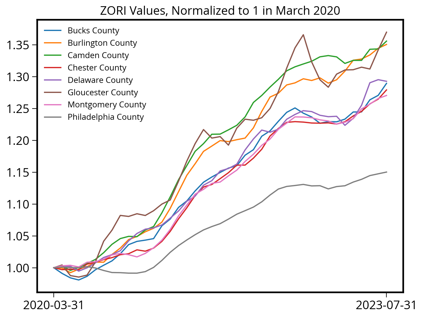

Plot the ZHVI values, normalized to 1 in March 2020:

# Create the figure and axes
fig, ax = plt.subplots()

# Iterate over the data, grouped by county name
for countyName, group_df in prices_philly_metro.groupby("RegionName"):
    
    # Trim to where Date > March 2020
    # Sort by Date in ascending order
    group_df = group_df.sort_values("Date").query("Date >= '2020-03-01'")

    # Date vs. ZHVI
    x = group_df["Date"]
    y = group_df["ZHVI"]
    
    # Trime
    ax.plot(x, y / y.iloc[0], label=countyName)

# Format and add a legend
ax.set_title("ZHVI Values, Normalized to 1 in March 2020")
ax.set_xticks(["2020-03-31", "2023-07-31"])
ax.legend(fontsize=10);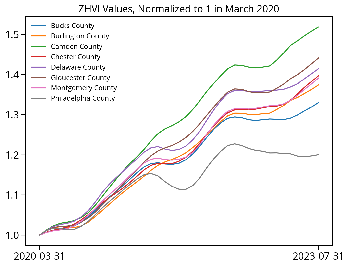

Takeaway: You can clearly see that price growth in Philadelphia significantly lags the growth in its suburb counties.

First Homework Assignment

Available on GitHub:

https://github.com/MUSA-550-Fall-2023/assignment-1

Two parts:

Download and install Python locally on your computer. Instructions in the assignment README!
Explore the “Donut Effect” using Zillow ZHVI data by ZIP code in Philadelphia, and submit your Jupyter notebook.

Important

Due date: Monday 9/25 by the end of the day (11:59 PM)

That’s it!

Next week: Data Visualization Fundamentals
Office hours:
- Nick: Mondays, 8:00PM - 10:00PM, remote
- Teresa: Fridays, 10:30AM - 12:00PM, remote
- Sign up for 15-minute time slots on Canvas (Zoom info in calendar invite)
Post any questions on Ed Discussion!
Email questions/concerns to nhand@design.upenn.edu

Today

Reminder: The weekly workflow

Python Data Analysis: the pandas package

The old logo

The new, less fun logo

Basic pandas concepts

1. Accessing data

2. Manipulating data

3. Applying a function

4. Data selection

Need more help?

A more interesting example: The Donut Effect

1. Population change

Exercise: Calculate the percent change in population for Philadelphia

2. Home & rental prices

Convert from “wide” to “tidy” format

Merge the data frames

Trim to the counties we want

Group by: split-apply-combine

Bonus: a matplotlib preview

First Homework Assignment

That’s it!

Bonus: a `matplotlib` preview