Week 11: Clustering Analysis in Python

from matplotlib import pyplot as plt
import numpy as np
import pandas as pd
import geopandas as gpd
np.random.seed(42)

Section 401
Nov 13, 2023

Clustering in Python

Both spatial and non-spatial datasets
Two new techniques:
- Non-spatial: K-means
- Spatial: DBSCAN
Two labs/exercises this week:
1. Grouping Philadelphia neighborhoods by AirBnb listings
2. Identifying clusters in taxi rides in NYC

“Machine learning” and “AI”

The computer learns patterns and properties of an input data set without the user specifying them beforehand
Can be both supervised and unsupervised

Supervised

Example: classification
Given a training set of labeled data, learn to assign labels to new data

Unsupervised

Example: clustering
Identify structure / clusters in data without any prior knowledge

Machine learning in Python: scikit-learn

State-of-the-art machine learning in Python
Easy to use, lots of functionality

Clustering is just one (of many) features

https://scikit-learn.org/stable/

Note

We will focus on clustering algorithms today and discuss a few other machine learning techniques in the next two weeks. If there is a specific scikit-learn use case we won’t cover, I’m open to ideas for incorporating it as part of the final project.

Part 1: Non-spatial clustering

The goal

Partition a dataset into groups that have a similar set of attributes, or features, within the group and a dissimilar set of features between groups.

Minimize the intra-cluster variance and maximize the inter-cluster variance of features.

Some intuition

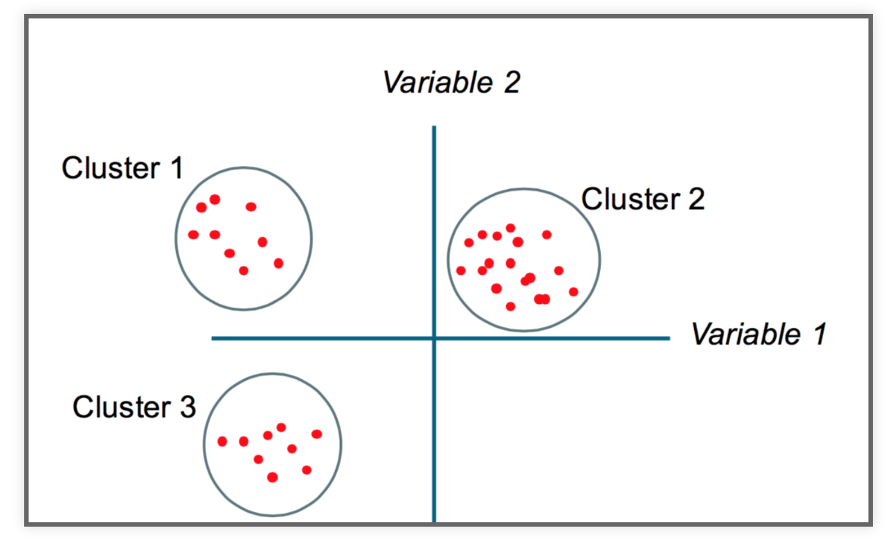
K-Means clustering

Simple but robust clustering algorithm
Widely used
Important: user must specify the number of clusters
Cannot be used to find density-based clusters

This is just one of several clustering methods

https://scikit-learn.org/stable/modules/clustering.html#overview-of-clustering-methods

A good introduction

Check out Andrew Ng’s Coursera lecture on unsupervised clustering.

How does it work?

Minimizes the intra-cluster variance: minimizes the sum of the squared distances between all points in a cluster and the cluster centroid

K-means in action

Example: Clustering countries by health and income

Health expectancy in years vs. GDP per capita and population for 187 countries (as of 2015)
Data from Gapminder

import altair as alt
from vega_datasets import data as vega_data

Read the data from a URL:

gapminder = pd.read_csv(vega_data.gapminder_health_income.url)
gapminder.head()

	country	income	health	population
0	Afghanistan	1925	57.63	32526562
1	Albania	10620	76.00	2896679
2	Algeria	13434	76.50	39666519
3	Andorra	46577	84.10	70473
4	Angola	7615	61.00	25021974

Plot it with altair:

(
    alt.Chart(gapminder)
    .mark_circle()
    .encode(
        alt.X("income:Q", scale=alt.Scale(type="log")),
        alt.Y("health:Q", scale=alt.Scale(zero=False)),
        size="population:Q",
        tooltip=list(gapminder.columns),
    )
    .properties(width=800, height=600)
    .interactive()
)

K-Means with scikit-learn

from sklearn.cluster import KMeans

Let’s start with 5 clusters

KMeans?

Init signature:
KMeans(
    n_clusters=8,
    *,
    init='k-means++',
    n_init='warn',
    max_iter=300,
    tol=0.0001,
    verbose=0,
    random_state=None,
    copy_x=True,
    algorithm='lloyd',
)
Docstring:     
K-Means clustering.
Read more in the :ref:`User Guide <k_means>`.
Parameters
----------
n_clusters : int, default=8
    The number of clusters to form as well as the number of
    centroids to generate.
init : {'k-means++', 'random'}, callable or array-like of shape             (n_clusters, n_features), default='k-means++'
    Method for initialization:
    'k-means++' : selects initial cluster centroids using sampling based on
    an empirical probability distribution of the points' contribution to the
    overall inertia. This technique speeds up convergence. The algorithm
    implemented is "greedy k-means++". It differs from the vanilla k-means++
    by making several trials at each sampling step and choosing the best centroid
    among them.
    'random': choose `n_clusters` observations (rows) at random from data
    for the initial centroids.
    If an array is passed, it should be of shape (n_clusters, n_features)
    and gives the initial centers.
    If a callable is passed, it should take arguments X, n_clusters and a
    random state and return an initialization.
n_init : 'auto' or int, default=10
    Number of times the k-means algorithm is run with different centroid
    seeds. The final results is the best output of `n_init` consecutive runs
    in terms of inertia. Several runs are recommended for sparse
    high-dimensional problems (see :ref:`kmeans_sparse_high_dim`).
    When `n_init='auto'`, the number of runs depends on the value of init:
    10 if using `init='random'` or `init` is a callable;
    1 if using `init='k-means++'` or `init` is an array-like.
    .. versionadded:: 1.2
       Added 'auto' option for `n_init`.
    .. versionchanged:: 1.4
       Default value for `n_init` will change from 10 to `'auto'` in version 1.4.
max_iter : int, default=300
    Maximum number of iterations of the k-means algorithm for a
    single run.
tol : float, default=1e-4
    Relative tolerance with regards to Frobenius norm of the difference
    in the cluster centers of two consecutive iterations to declare
    convergence.
verbose : int, default=0
    Verbosity mode.
random_state : int, RandomState instance or None, default=None
    Determines random number generation for centroid initialization. Use
    an int to make the randomness deterministic.
    See :term:`Glossary <random_state>`.
copy_x : bool, default=True
    When pre-computing distances it is more numerically accurate to center
    the data first. If copy_x is True (default), then the original data is
    not modified. If False, the original data is modified, and put back
    before the function returns, but small numerical differences may be
    introduced by subtracting and then adding the data mean. Note that if
    the original data is not C-contiguous, a copy will be made even if
    copy_x is False. If the original data is sparse, but not in CSR format,
    a copy will be made even if copy_x is False.
algorithm : {"lloyd", "elkan", "auto", "full"}, default="lloyd"
    K-means algorithm to use. The classical EM-style algorithm is `"lloyd"`.
    The `"elkan"` variation can be more efficient on some datasets with
    well-defined clusters, by using the triangle inequality. However it's
    more memory intensive due to the allocation of an extra array of shape
    `(n_samples, n_clusters)`.
    `"auto"` and `"full"` are deprecated and they will be removed in
    Scikit-Learn 1.3. They are both aliases for `"lloyd"`.
    .. versionchanged:: 0.18
        Added Elkan algorithm
    .. versionchanged:: 1.1
        Renamed "full" to "lloyd", and deprecated "auto" and "full".
        Changed "auto" to use "lloyd" instead of "elkan".
Attributes
----------
cluster_centers_ : ndarray of shape (n_clusters, n_features)
    Coordinates of cluster centers. If the algorithm stops before fully
    converging (see ``tol`` and ``max_iter``), these will not be
    consistent with ``labels_``.
labels_ : ndarray of shape (n_samples,)
    Labels of each point
inertia_ : float
    Sum of squared distances of samples to their closest cluster center,
    weighted by the sample weights if provided.
n_iter_ : int
    Number of iterations run.
n_features_in_ : int
    Number of features seen during :term:`fit`.
    .. versionadded:: 0.24
feature_names_in_ : ndarray of shape (`n_features_in_`,)
    Names of features seen during :term:`fit`. Defined only when `X`
    has feature names that are all strings.
    .. versionadded:: 1.0
See Also
--------
MiniBatchKMeans : Alternative online implementation that does incremental
    updates of the centers positions using mini-batches.
    For large scale learning (say n_samples > 10k) MiniBatchKMeans is
    probably much faster than the default batch implementation.
Notes
-----
The k-means problem is solved using either Lloyd's or Elkan's algorithm.
The average complexity is given by O(k n T), where n is the number of
samples and T is the number of iteration.
The worst case complexity is given by O(n^(k+2/p)) with
n = n_samples, p = n_features.
Refer to :doi:`"How slow is the k-means method?" D. Arthur and S. Vassilvitskii -
SoCG2006.<10.1145/1137856.1137880>` for more details.
In practice, the k-means algorithm is very fast (one of the fastest
clustering algorithms available), but it falls in local minima. That's why
it can be useful to restart it several times.
If the algorithm stops before fully converging (because of ``tol`` or
``max_iter``), ``labels_`` and ``cluster_centers_`` will not be consistent,
i.e. the ``cluster_centers_`` will not be the means of the points in each
cluster. Also, the estimator will reassign ``labels_`` after the last
iteration to make ``labels_`` consistent with ``predict`` on the training
set.
Examples
--------
>>> from sklearn.cluster import KMeans
>>> import numpy as np
>>> X = np.array([[1, 2], [1, 4], [1, 0],
...               [10, 2], [10, 4], [10, 0]])
>>> kmeans = KMeans(n_clusters=2, random_state=0, n_init="auto").fit(X)
>>> kmeans.labels_
array([1, 1, 1, 0, 0, 0], dtype=int32)
>>> kmeans.predict([[0, 0], [12, 3]])
array([1, 0], dtype=int32)
>>> kmeans.cluster_centers_
array([[10.,  2.],
       [ 1.,  2.]])
File:           ~/mambaforge/envs/musa-550-fall-2023/lib/python3.10/site-packages/sklearn/cluster/_kmeans.py
Type:           ABCMeta
Subclasses:

kmeans = KMeans(n_clusters=5, n_init=10)

Lot’s of optional parameters, but n_clusters is the most important:

Let’s fit just income first

Use the fit() function

kmeans.fit(gapminder[['income']]);

Extract the cluster labels

Use the labels_ attribute

gapminder['label'] = kmeans.labels_

How big are our clusters?

gapminder.groupby('label').size()

label
0    106
1      6
2     50
3      1
4     24
dtype: int64

Plot it again, coloring by our labels

(
    alt.Chart(gapminder)
    .mark_circle()
    .encode(
        alt.X("income:Q", scale=alt.Scale(type="log")),
        alt.Y("health:Q", scale=alt.Scale(zero=False)),
        size="population:Q",
        color=alt.Color("label:N", scale=alt.Scale(scheme="dark2")),
        tooltip=list(gapminder.columns),
    )
    .properties(width=800, height=600)
    .interactive()
)

Calculate average income by group

gapminder.groupby("label")['income'].mean().sort_values()

label
0      5279.830189
2     21040.820000
4     42835.500000
1     74966.166667
3    132877.000000
Name: income, dtype: float64

Data is nicely partitioned into income levels

How about health, income, and population?

# Fit all three columns
kmeans.fit(gapminder[['income', 'health', 'population']])

# Extract the labels
gapminder['label'] = kmeans.labels_

gapminder

	country	income	health	population	label
0	Afghanistan	1925	57.63	32526562	2
1	Albania	10620	76.00	2896679	2
2	Algeria	13434	76.50	39666519	0
3	Andorra	46577	84.10	70473	2
4	Angola	7615	61.00	25021974	2
...	...	...	...	...	...
182	Vietnam	5623	76.50	93447601	0
183	West Bank and Gaza	4319	75.20	4668466	2
184	Yemen	3887	67.60	26832215	2
185	Zambia	4034	58.96	16211767	2
186	Zimbabwe	1801	60.01	15602751	2

187 rows × 5 columns

(
    alt.Chart(gapminder)
    .mark_circle()
    .encode(
        alt.X("income:Q", scale=alt.Scale(type="log")),
        alt.Y("health:Q", scale=alt.Scale(zero=False)),
        size="population:Q",
        color=alt.Color("label:N", scale=alt.Scale(scheme="dark2")),
        tooltip=list(gapminder.columns),
    )
    .properties(width=800, height=600)
    .interactive()
)

It….didn’t work that well

What’s wrong?

K-means is distance-based, but our features have wildly different distance scales

scikit-learn to the rescue: pre-processing

Scikit-learn has a utility to normalize features with an average of zero and a variance of 1
Use the StandardScaler class

from sklearn.preprocessing import MinMaxScaler, RobustScaler

from sklearn.preprocessing import StandardScaler

scaler = StandardScaler()

Use the `fit_transform()` function to scale your features

gapminder_scaled = scaler.fit_transform(gapminder[['income', 'health', 'population']])

Important: The fit_transform() function converts the DataFrame to a numpy array:

# fit_transform() converts the data into a numpy array
gapminder_scaled[:5]

array([[-0.79481258, -1.8171424 , -0.04592039],
       [-0.34333373,  0.55986273, -0.25325837],
       [-0.1972197 ,  0.62456075,  0.00404216],
       [ 1.52369617,  1.6079706 , -0.27303503],
       [-0.49936524, -1.38107777, -0.09843447]])

# mean of zero
gapminder_scaled.mean(axis=0)

array([ 8.07434927e-17, -1.70511258e-15, -1.89984689e-17])

# variance of one
gapminder_scaled.std(axis=0)

array([1., 1., 1.])

Now fit the scaled features

# Perform the fit
kmeans.fit(gapminder_scaled)

# Extract the labels
gapminder['label'] = kmeans.labels_

(
    alt.Chart(gapminder)
    .mark_circle()
    .encode(
        alt.X("income:Q", scale=alt.Scale(type="log")),
        alt.Y("health:Q", scale=alt.Scale(zero=False)),
        size="population:Q",
        color=alt.Color("label:N", scale=alt.Scale(scheme="dark2")),
        tooltip=list(gapminder.columns),
    )
    .properties(width=800, height=600)
    .interactive()
)

# Number of countries per cluster
gapminder.groupby("label").size()

label
0    62
1    85
2     5
3     2
4    33
dtype: int64

# Average population per cluster
gapminder.groupby("label")['population'].mean().sort_values() / 1e6

label
2       2.544302
0      21.191274
1      26.478761
4      31.674060
3    1343.549735
Name: population, dtype: float64

# Average life expectancy per cluster
gapminder.groupby("label")['health'].mean().sort_values()

label
0    62.342097
3    71.850000
1    74.376353
4    80.830303
2    80.920000
Name: health, dtype: float64

# Average income per cluster
gapminder.groupby("label")['income'].mean().sort_values() / 1e3

label
0     4.136016
3     9.618500
1    13.347376
4    41.048818
2    91.524200
Name: income, dtype: float64

gapminder.loc[gapminder['label']==4]

	country	income	health	population	label
3	Andorra	46577	84.1	70473	4
8	Australia	44056	81.8	23968973	4
9	Austria	44401	81.0	8544586	4
12	Bahrain	44138	79.2	1377237	4
16	Belgium	41240	80.4	11299192	4
30	Canada	43294	81.7	35939927	4
44	Cyprus	29797	82.6	1165300	4
45	Czech Republic	29437	78.6	10543186	4
46	Denmark	43495	80.1	5669081	4
58	Finland	38923	80.8	5503457	4
59	France	37599	81.9	64395345	4
63	Germany	44053	81.1	80688545	4
65	Greece	25430	79.8	10954617	4
74	Iceland	42182	82.8	329425	4
79	Ireland	47758	80.4	4688465	4
80	Israel	31590	82.4	8064036	4
81	Italy	33297	82.1	59797685	4
83	Japan	36162	83.5	126573481	4
104	Malta	30265	82.1	418670	4
118	Netherlands	45784	80.6	16924929	4
119	New Zealand	34186	80.6	4528526	4
124	Norway	64304	81.6	5210967	4
125	Oman	48226	75.7	4490541	4
133	Portugal	26437	79.8	10349803	4
140	Saudi Arabia	52469	78.1	31540372	4
147	Slovenia	28550	80.2	2067526	4
151	South Korea	34644	80.7	50293439	4
153	Spain	32979	81.7	46121699	4
160	Sweden	44892	82.0	9779426	4
161	Switzerland	56118	82.9	8298663	4
175	United Arab Emirates	60749	76.6	9156963	4
176	United Kingdom	38225	81.4	64715810	4
177	United States	53354	79.1	321773631	4

kmeans.inertia_

80.72009578392847

gapminder.loc[gapminder['label']==4]

	country	income	health	population	label
3	Andorra	46577	84.1	70473	4
8	Australia	44056	81.8	23968973	4
9	Austria	44401	81.0	8544586	4
12	Bahrain	44138	79.2	1377237	4
16	Belgium	41240	80.4	11299192	4
30	Canada	43294	81.7	35939927	4
44	Cyprus	29797	82.6	1165300	4
45	Czech Republic	29437	78.6	10543186	4
46	Denmark	43495	80.1	5669081	4
58	Finland	38923	80.8	5503457	4
59	France	37599	81.9	64395345	4
63	Germany	44053	81.1	80688545	4
65	Greece	25430	79.8	10954617	4
74	Iceland	42182	82.8	329425	4
79	Ireland	47758	80.4	4688465	4
80	Israel	31590	82.4	8064036	4
81	Italy	33297	82.1	59797685	4
83	Japan	36162	83.5	126573481	4
104	Malta	30265	82.1	418670	4
118	Netherlands	45784	80.6	16924929	4
119	New Zealand	34186	80.6	4528526	4
124	Norway	64304	81.6	5210967	4
125	Oman	48226	75.7	4490541	4
133	Portugal	26437	79.8	10349803	4
140	Saudi Arabia	52469	78.1	31540372	4
147	Slovenia	28550	80.2	2067526	4
151	South Korea	34644	80.7	50293439	4
153	Spain	32979	81.7	46121699	4
160	Sweden	44892	82.0	9779426	4
161	Switzerland	56118	82.9	8298663	4
175	United Arab Emirates	60749	76.6	9156963	4
176	United Kingdom	38225	81.4	64715810	4
177	United States	53354	79.1	321773631	4

Exercise: Clustering neighborhoods by Airbnb stats

I’ve extracted neighborhood Airbnb statistics for Philadelphia neighborhoods from Tom Slee’s website.

The data includes average price per person, overall satisfaction, and number of listings.

Two good references for Airbnb data

Original research study: How Airbnb’s Data Hid the Facts in New York City

Step 1: Load the data with pandas

The data is available in CSV format (“philly_airbnb_by_neighborhoods.csv”) in the “data/” folder of the repository.

airbnb = pd.read_csv("data/philly_airbnb_by_neighborhoods.csv")
airbnb.head()

	neighborhood	price_per_person	overall_satisfaction	N
0	ALLEGHENY_WEST	120.791667	4.666667	23
1	BELLA_VISTA	87.407920	3.158333	204
2	BELMONT	69.425000	3.250000	11
3	BREWERYTOWN	71.788188	1.943182	142
4	BUSTLETON	55.833333	1.250000	19

Step 2: Perform the K-Means fit

Use our three features: price_per_person, overall_satisfaction, N
I used 5 clusters, but you are welcome to experiment with different values! We will discuss what the optimal number is after we go through the solutions!
Scaling the features is recommended, but if the scales aren’t too different, so probably isn’t necessary in this case

# Initialize the Kmeans object
kmeans = KMeans(n_clusters=5, random_state=42, n_init=10)

Pre-process the data:

# Scale the data features we want
scaler = StandardScaler()
scaled_airbnb_data = scaler.fit_transform(airbnb[['price_per_person', 'overall_satisfaction', 'N']])

scaled_airbnb_data[:5]

array([[ 0.79001045,  1.74917003, -0.52348653],
       [ 0.0714296 ,  0.41880366,  0.40700931],
       [-0.31565045,  0.49965466, -0.58517687],
       [-0.26478314, -0.65297315,  0.08827593],
       [-0.60820933, -1.26436704, -0.54404998]])

# Run the fit! This adds the ".labels_" attribute
kmeans.fit(scaled_airbnb_data);

kmeans.labels_

array([0, 0, 0, 0, 1, 0, 0, 0, 0, 0, 0, 0, 0, 0, 0, 0, 4, 0, 0, 4, 4, 0,
       1, 4, 0, 0, 0, 0, 0, 0, 0, 0, 0, 0, 0, 4, 0, 0, 1, 0, 0, 0, 0, 1,
       0, 1, 0, 4, 0, 0, 0, 0, 1, 0, 0, 0, 0, 4, 0, 0, 4, 0, 0, 1, 1, 1,
       0, 0, 0, 1, 4, 0, 4, 1, 0, 3, 0, 0, 2, 4, 1, 0, 4, 4, 0, 1, 1, 0,
       4, 0, 0, 4, 0, 1, 0, 0, 0, 0, 0, 1, 1, 0, 0, 1, 1], dtype=int32)

# Save the cluster labels
airbnb["label"] = kmeans.labels_

# New column "label"!
airbnb.head()

	neighborhood	price_per_person	overall_satisfaction	N	label
0	ALLEGHENY_WEST	120.791667	4.666667	23	0
1	BELLA_VISTA	87.407920	3.158333	204	0
2	BELMONT	69.425000	3.250000	11	0
3	BREWERYTOWN	71.788188	1.943182	142	0
4	BUSTLETON	55.833333	1.250000	19	1

Step 3: Calculate average features per cluster

To gain some insight into our clusters, after calculating the K-Means labels: - group by the label column - calculate the mean() of each of our features - calculate the number of neighborhoods per cluster

airbnb.groupby('label', as_index=False).size()

	label	size
0	0	69
1	1	19
2	2	1
3	3	1
4	4	15

airbnb.groupby("label", as_index=False)[
    ["price_per_person", "overall_satisfaction", "N"]
].mean().sort_values(by="price_per_person")

	label	price_per_person	overall_satisfaction	N
0	0	73.199020	3.137213	76.550725
1	1	79.250011	0.697461	23.473684
4	4	116.601261	2.936508	389.933333
3	3	136.263996	3.000924	1499.000000
2	2	387.626984	5.000000	31.000000

airbnb.loc[airbnb['label'] == 2]

	neighborhood	price_per_person	overall_satisfaction	N	label
78	SHARSWOOD	387.626984	5.0	31	2

airbnb.loc[airbnb['label'] == 3]

	neighborhood	price_per_person	overall_satisfaction	N	label
75	RITTENHOUSE	136.263996	3.000924	1499	3

airbnb.loc[airbnb['label'] == 4]

	neighborhood	price_per_person	overall_satisfaction	N	label
16	EAST_PARK	193.388889	2.714286	42	4
19	FAIRMOUNT	144.764110	2.903614	463	4
20	FISHTOWN	59.283468	2.963816	477	4
23	FRANCISVILLE	124.795795	3.164062	300	4
35	GRADUATE_HOSPITAL	106.420417	3.180791	649	4
47	LOGAN_SQUARE	145.439414	3.139241	510	4
57	NORTHERN_LIBERTIES	145.004866	3.095506	367	4
60	OLD_CITY	111.708084	2.756637	352	4
70	POINT_BREEZE	63.801072	2.759542	435	4
72	QUEEN_VILLAGE	106.405744	3.125000	248	4
79	SOCIETY_HILL	133.598667	3.118421	165	4
82	SPRING_GARDEN	157.125692	3.454023	413	4
83	SPRUCE_HILL	48.095512	2.377358	399	4
88	UNIVERSITY_CITY	82.228062	2.231579	326	4
91	WASHINGTON_SQUARE	126.959118	3.063745	703	4

Step 4: Plot a choropleth, coloring neighborhoods by their cluster label

Part 1: Load the Philadelphia neighborhoods available in the data directory:
- ./data/philly_neighborhoods.geojson
Part 2: Merge the Airbnb data (with labels) and the neighborhood polygons
Part 3: Use geopandas to plot the neighborhoods
- The categorical=True and legend=True keywords will be useful here

hoods = gpd.read_file("./data/philly_neighborhoods.geojson")
hoods.head()

	Name	geometry
0	LAWNDALE	POLYGON ((-75.08616 40.05013, -75.08893 40.044...
1	ASTON_WOODBRIDGE	POLYGON ((-75.00860 40.05369, -75.00861 40.053...
2	CARROLL_PARK	POLYGON ((-75.22673 39.97720, -75.22022 39.974...
3	CHESTNUT_HILL	POLYGON ((-75.21278 40.08637, -75.21272 40.086...
4	BURNHOLME	POLYGON ((-75.08768 40.06861, -75.08758 40.068...

airbnb.head()

	neighborhood	price_per_person	overall_satisfaction	N	label
0	ALLEGHENY_WEST	120.791667	4.666667	23	0
1	BELLA_VISTA	87.407920	3.158333	204	0
2	BELMONT	69.425000	3.250000	11	0
3	BREWERYTOWN	71.788188	1.943182	142	0
4	BUSTLETON	55.833333	1.250000	19	1

# Do the merge
# Note: how='left' will keep ALL of the geometries, even if they don't have any AirBnB data
airbnb2 = hoods.merge(airbnb, left_on='Name', right_on='neighborhood', how='left')

# Some neigborhoods don't have listings and get assigned the NaN label
# Assign -1 to the neighborhoods without any listings instead
airbnb2['label'] = airbnb2['label'].fillna(-1)

# plot the data
airbnb2 = airbnb2.to_crs(epsg=3857)

# setup the figure
f, ax = plt.subplots(figsize=(10, 8))

# plot, coloring by label column
# specify categorical data and add legend
airbnb2.plot(
    column="label",
    cmap="Dark2",
    categorical=True,
    legend=True,
    edgecolor="k",
    lw=0.5,
    ax=ax,
)


ax.set_axis_off()
plt.axis("equal");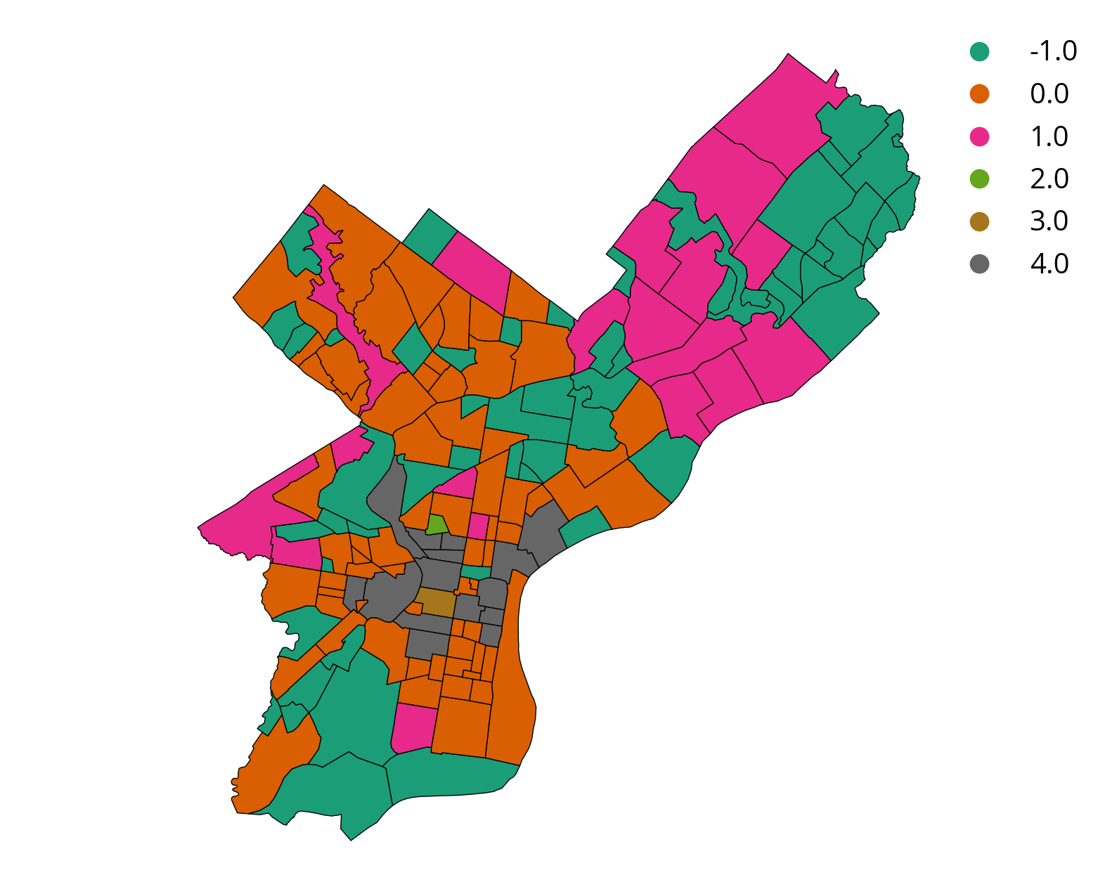

Step 5: Plot an interactive map

Use hvplot / geopandas to plot the clustering results with a tooltip for neighborhood name and tooltip.

airbnb2.explore(
    column="label",
    cmap="Dark2",
    categorical=True,
    legend=True,
    tiles="CartoDB positron"
)

Make this Notebook Trusted to load map: File -> Trust Notebook

Based on these results, where would you want to stay?

Group 0!

Why 5 groups?

Use the “Elbow” method…

# Number of clusters to try out
n_clusters = list(range(2, 10))

# Run kmeans for each value of k
inertias = []
for k in n_clusters:
    
    # Initialize and run
    kmeans = KMeans(n_clusters=k, n_init=10)
    kmeans.fit(scaled_airbnb_data)
    
    # Save the "inertia"
    inertias.append(kmeans.inertia_)
    
# Plot it!
plt.plot(n_clusters, inertias, marker='o', ms=10, mfc='white', lw=4, mew=3);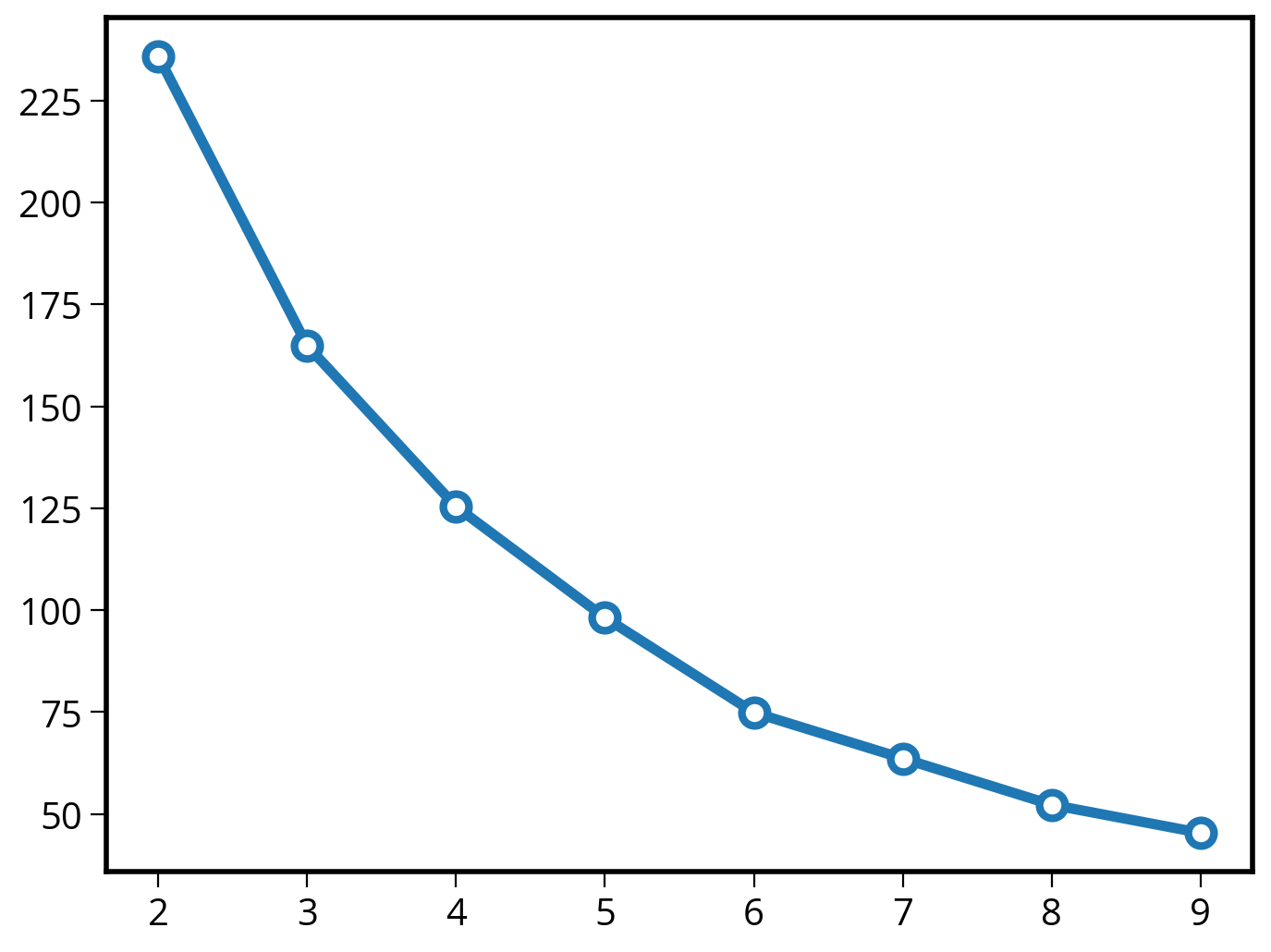

The `kneed` package

There is also a nice package called kneed that can determine the “knee” point quantitatively, using the kneedle algorithm.

n_clusters

[2, 3, 4, 5, 6, 7, 8, 9]

from kneed import KneeLocator

# Initialize the knee algorithm
kn = KneeLocator(n_clusters, inertias, curve='convex', direction='decreasing')

# Print out the knee 
print(kn.knee)

That’s it!

More clustering on Wednesday!

Clustering in Python

“Machine learning” and “AI”

Supervised

Unsupervised

Machine learning in Python: scikit-learn

Clustering is just one (of many) features

Part 1: Non-spatial clustering

Some intuition

K-Means clustering

This is just one of several clustering methods

How does it work?

K-means in action

Example: Clustering countries by health and income

K-Means with scikit-learn

Let’s fit just income first

Extract the cluster labels

How big are our clusters?

Plot it again, coloring by our labels

Calculate average income by group

How about health, income, and population?

It….didn’t work that well

scikit-learn to the rescue: pre-processing

Use the fit_transform() function to scale your features

Now fit the scaled features

Exercise: Clustering neighborhoods by Airbnb stats

Step 1: Load the data with pandas

Step 2: Perform the K-Means fit

Step 3: Calculate average features per cluster

Step 4: Plot a choropleth, coloring neighborhoods by their cluster label

Step 5: Plot an interactive map

Based on these results, where would you want to stay?

Why 5 groups?

The kneed package

That’s it!

Use the `fit_transform()` function to scale your features

The `kneed` package