Week 12B: Predictive modeling with scikit-learn

from matplotlib import pyplot as plt
import numpy as np
import pandas as pd
import geopandas as gpd
import hvplot.pandas

np.random.seed(42)

pd.options.display.max_columns = 999

%matplotlib inline

• Nov 27, 2023
• Section 401

The plan for today

• Wrap up our money vs. happiness example
• Introduce decision trees and random forests
• Case study: Modeling housing prices in Philadelphia

Supervised learning with scikit-learn

Example: does money make people happier?

We’ll load data compiled from two data sources: - The Better Life Index from the OECD’s website - GDP per capita from the IMF’s website

# Load the data 
data = pd.read_csv("./data/gdp_vs_satisfaction.csv")
data.head()

	Country	life_satisfaction	gdp_per_capita
0	Australia	7.3	50961.87
1	Austria	7.1	43724.03
2	Belgium	6.9	40106.63
3	Brazil	6.4	8670.00
4	Canada	7.4	43331.96

# Linear models
from sklearn.linear_model import LinearRegression
from sklearn.linear_model import Ridge

# Model selection
from sklearn.model_selection import train_test_split

# Pipelines
from sklearn.pipeline import make_pipeline

# Preprocessing
from sklearn.preprocessing import StandardScaler
from sklearn.preprocessing import PolynomialFeatures

First step: set up the test/train split of input data:

# Do a 70/30 train/test split
train_set, test_set = train_test_split(data, test_size=0.3, random_state=42)

# Features
X_train = train_set['gdp_per_capita'].values
X_train = X_train[:, np.newaxis]

X_test = test_set['gdp_per_capita'].values
X_test = X_test[:, np.newaxis]

# Labels
y_train = train_set['life_satisfaction'].values
y_test = test_set['life_satisfaction'].values

Where we left off: overfitting

As we increase the polynomial degree (add more and more polynomial features) two things happen:

1. Training accuracy goes way up
2. Test accuracy goes way down

This is the classic case of overfitting — our model does not generalize well at all.

Regularization to the rescue?

• The Ridge adds regularization to the linear regression least squares model
• Parameter alpha determines the level of regularization
• Larger values of alpha mean stronger regularization — results in a “simpler” bestfit

Remember, regularization penalizes large parameter values and complex fits

Let’s gain some intuition:

• Fix the polynomial degree to 3
• Try out alpha values of 0, 10, 100, and \(10^5\)
• Compare to linear fit (no polynomial features)

Important - Baseline: linear model - This uses LinearModel and scales input features with StandardScaler - Ridge regression: try multiple regularization strength values - Use a pipeline object to apply both a StandardScaler and PolynomialFeatures(degree=3) pre-processing to features

Set up a grid of GDP per capita points to make predictions for:

# The values we want to predict (ranging from our min to max GDP per capita)
gdp_pred = np.linspace(1e3, 1.1e5, 100)

# Sklearn needs the second axis!
X_pred = gdp_pred[:, np.newaxis]

# Create a pre-processing pipeline
# This scales and adds polynomial features up to degree = 3
pipe = make_pipeline(StandardScaler(), PolynomialFeatures(degree=3))

# BASELINE: Setup and fit a linear model (with scaled features)
linear = LinearRegression()
scaler = StandardScaler()
linear.fit(scaler.fit_transform(X_train), y_train)


with plt.style.context("fivethirtyeight"):

    fig, ax = plt.subplots(figsize=(10, 6))

    ## Plot the data
    ax.scatter(
        data["gdp_per_capita"] / 1e5,
        data["life_satisfaction"],
        label="Data",
        s=100,
        zorder=10,
        color="#666666",
    )

    ## Evaluate the linear fit
    print("Linear fit")
    training_score = linear.score(scaler.fit_transform(X_train), y_train)
    print(f"Training Score = {training_score}")

    test_score = linear.score(scaler.fit_transform(X_test), y_test)
    print(f"Test Score = {test_score}")
    print()


    ## Plot the linear fit
    ax.plot(
        X_pred / 1e5,
        linear.predict(scaler.fit_transform(X_pred)),
        color="k",
        label="Linear fit",
    )

    ## Ridge regression: linear model with regularization 
    # Plot the predicted values for each alpha
    for alpha in [0, 10, 100, 1e5]:
        print(f"alpha = {alpha}")

        # Create out Ridge model with this alpha
        ridge = Ridge(alpha=alpha)

        # Fit the model on the training set
        # NOTE: Use the pipeline that includes polynomial features
        ridge.fit(pipe.fit_transform(X_train), y_train)

        # Evaluate on the training set
        training_score = ridge.score(pipe.fit_transform(X_train), y_train)
        print(f"Training Score = {training_score}")

        # Evaluate on the test set
        test_score = ridge.score(pipe.fit_transform(X_test), y_test)
        print(f"Test Score = {test_score}")

        # Plot the ridge results
        y_pred = ridge.predict(pipe.fit_transform(X_pred))
        ax.plot(X_pred / 1e5, y_pred, label=f"alpha = {alpha}")

        print()

    # Plot formatting
    ax.legend(ncol=2, loc=0)
    ax.set_ylim(4, 8)
    ax.set_xlabel("GDP Per Capita ($\\times$ $10^5$)")
    ax.set_ylabel("Life Satisfaction")

Linear fit
Training Score = 0.4638100579740343
Test Score = 0.35959585147159556

alpha = 0
Training Score = 0.6458898101593082
Test Score = 0.5597457659851048

alpha = 10
Training Score = 0.5120282691427858
Test Score = 0.38335642103788325

alpha = 100
Training Score = 0.1815398751108913
Test Score = -0.05242399995626967

alpha = 100000.0
Training Score = 0.0020235571180508005
Test Score = -0.26129559971586125

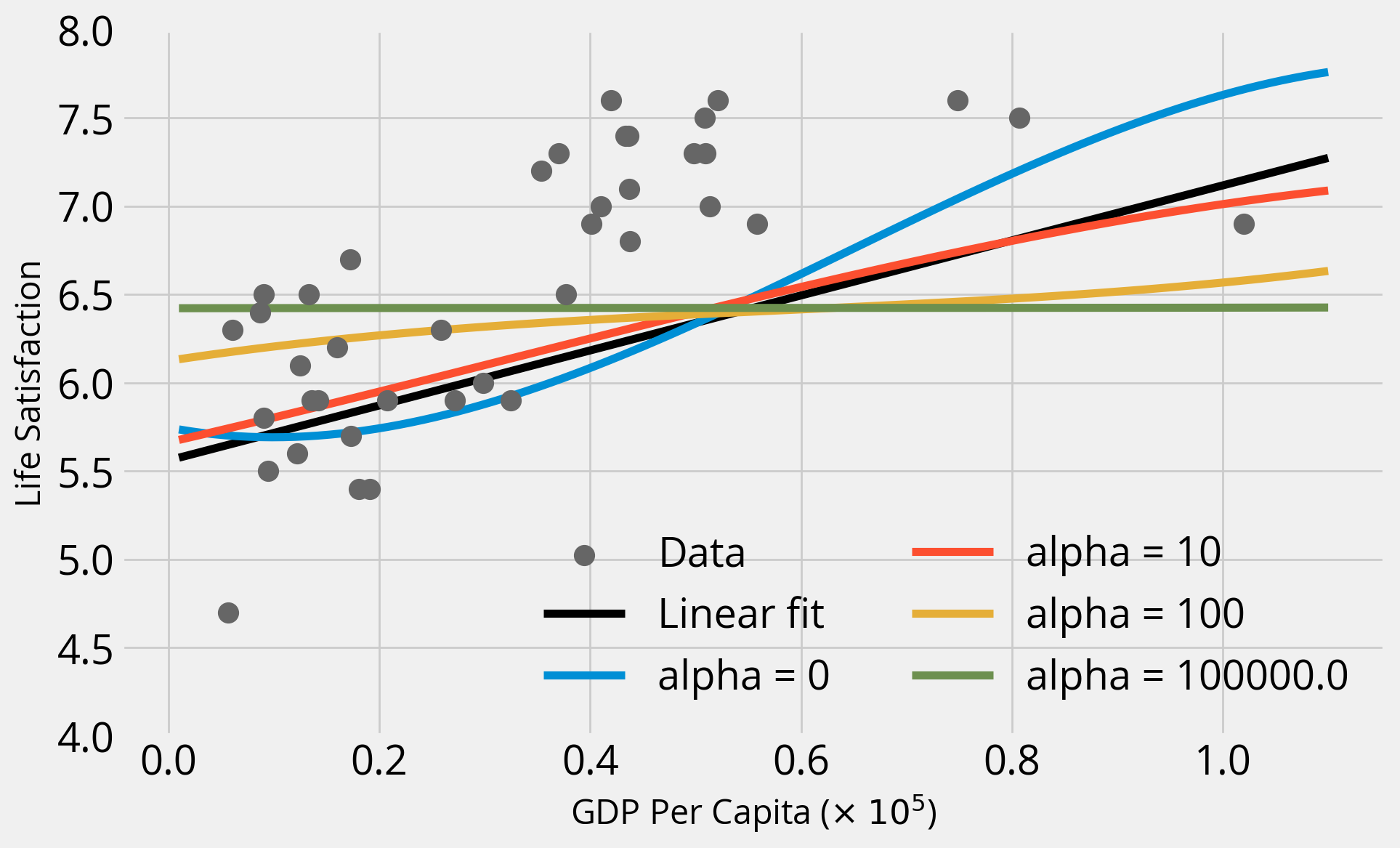
Takeaways

• As we increase alpha, the fits become “simpler” and coefficients get closer and closer to zero — a straight line!
• When alpha = 0 (no regularization), we get the same result as when we ran LinearRegression() with the polynomial features
• In this case, regularization doesn’t improve the fit, and the base polynomial regression (degree=3) provides the best fit

Recap: what we learned so far

• The LinearRegression model
• The test/train split and evaluation
• Feature engineering: scaling and creating polynomial features
• The Ridge model and regularization
• Creating Pipeline() objects

How can we improve?

More feature engineering!

In this case, I’ve done the hard work for you and pulled additional country properties from the OECD’s website.

data2 = pd.read_csv("./data/gdp_vs_satisfaction_more_features.csv")

data2.head()

	Country	life_satisfaction	GDP per capita	Air pollution	Employment rate	Feeling safe walking alone at night	Homicide rate	Life expectancy	Quality of support network	Voter turnout	Water quality
0	Australia	7.3	50961.87	5.0	73.0	63.5	1.1	82.5	95.0	91.0	93.0
1	Austria	7.1	43724.03	16.0	72.0	80.6	0.5	81.7	92.0	80.0	92.0
2	Belgium	6.9	40106.63	15.0	63.0	70.1	1.0	81.5	91.0	89.0	84.0
3	Brazil	6.4	8670.00	10.0	61.0	35.6	26.7	74.8	90.0	79.0	73.0
4	Canada	7.4	43331.96	7.0	73.0	82.2	1.3	81.9	93.0	68.0	91.0

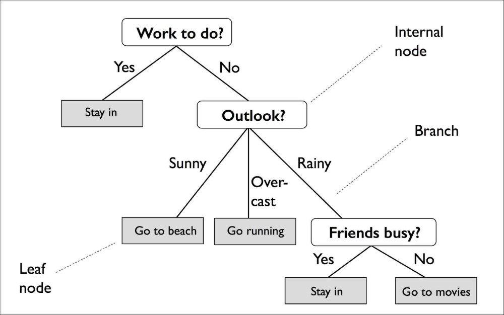
Decision trees: a more sophisticated modeling algorithm

We’ll move beyond simple linear regression and see if we can get a better fit.

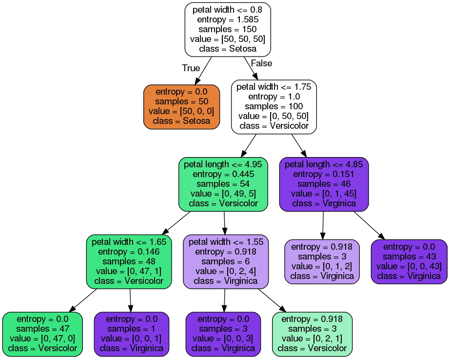
A decision tree learns decision rules from the input features:

A decision tree classifier for the Iris data set

More info on the iris data set

Regression with decision trees is similar

For a specific corner of the input feature space, the decision tree predicts an output target value

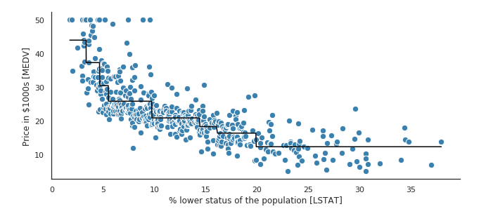
Decision trees suffer from overfitting

Decision trees can be very deep with many nodes — this will lead to overfitting your dataset!

Random forests: an ensemble solution to overfitting

• Introduces randomization into the fitting process to avoid overfitting
• Fits multiple decision trees on random subsets of the input data
• Avoids overfitting and leads to better overall fits

This is an example of ensemble learning: combining multiple estimators to achieve better overall accuracy than any one model could achieve

from sklearn.ensemble import RandomForestRegressor

Let’s split our data into training and test sets again:

# Split the data 70/30
train_set, test_set = train_test_split(data2, test_size=0.3, random_state=42)

# the target labels
y_train = train_set["life_satisfaction"].values
y_test = test_set["life_satisfaction"].values

# The features
feature_cols = [col for col in data2.columns if col not in ["life_satisfaction", "Country"]]
X_train = train_set[feature_cols].values
X_test = test_set[feature_cols].values

feature_cols

['GDP per capita',
 'Air pollution',
 'Employment rate',
 'Feeling safe walking alone at night',
 'Homicide rate',
 'Life expectancy',
 'Quality of support network',
 'Voter turnout',
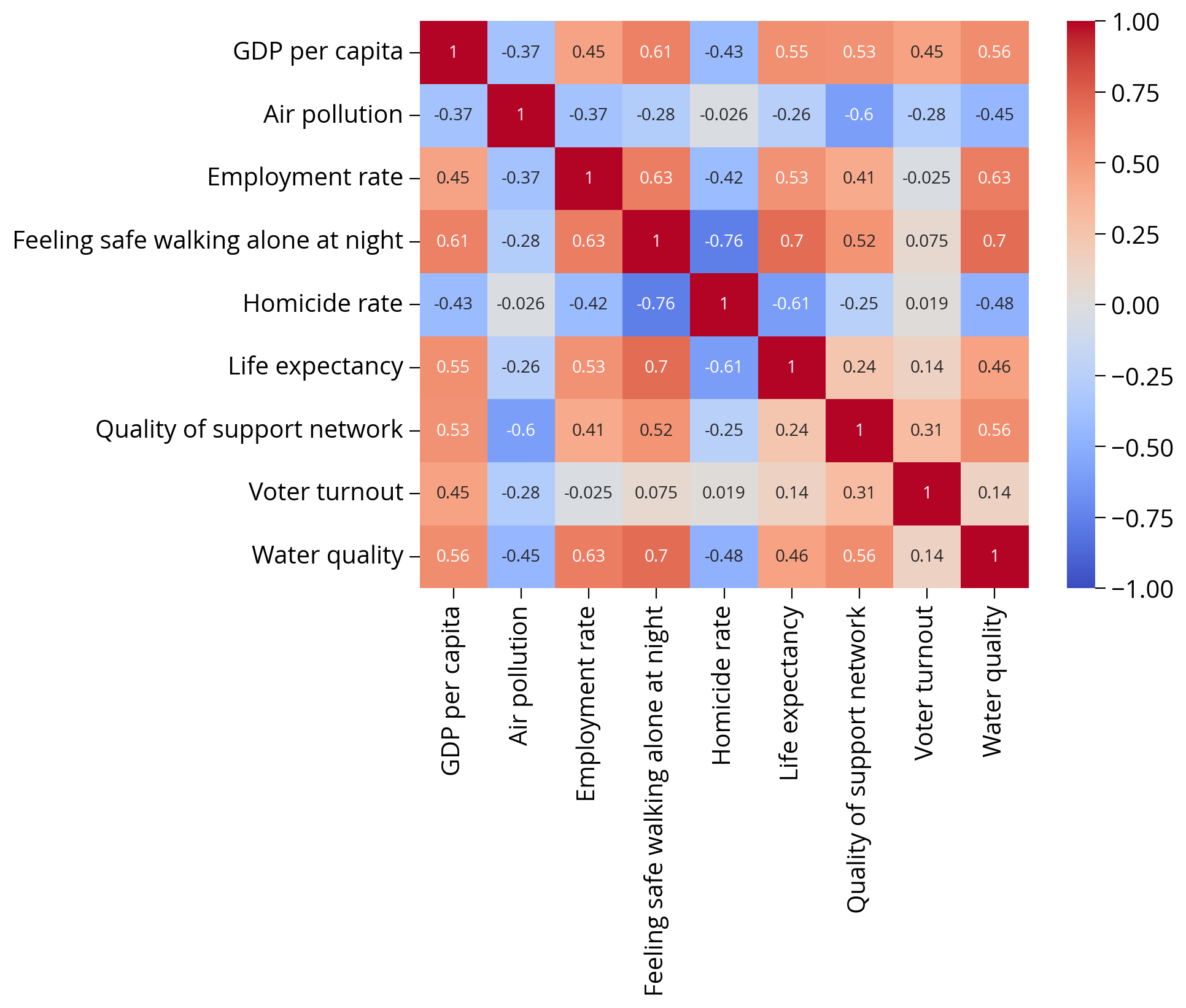
 'Water quality']

Let’s check for correlations in our input data

• Highly correlated input variables can skew the model fits and lead to worse accuracy
• Best to remove features with high correlations (rule of thumb: coefficients > 0.7 or 0.8, typically)

import seaborn as sns

sns.heatmap(
    train_set[feature_cols].corr(), 
    cmap="coolwarm", 
    annot=True, 
    vmin=-1, 
    vmax=1
);

Let’s do some fitting…

New: Pipelines support models as the last step!

• Very useful for setting up reproducible machine learning analyses!
• The Pipeline behaves just like a model, but it runs the transformations beforehand
• Simplifies the analysis: now we can just call the .fit() function of the pipeline instead of the model

Establish a baseline with a linear model:

# Linear model pipeline with two steps
linear_pipe = make_pipeline(StandardScaler(), LinearRegression())

# Fit the pipeline
# NEW: This applies all of the transformations, and then fits the model
print("Linear regression")
linear_pipe.fit(X_train, y_train)

# NEW: Print the training score
training_score = linear_pipe.score(X_train, y_train)
print(f"Training Score = {training_score}")

# NEW: Print the test score
test_score = linear_pipe.score(X_test, y_test)
print(f"Test Score = {test_score}")

Linear regression
Training Score = 0.755333265746168
Test Score = 0.6478865590446827

Now fit a random forest:

# Random forest model pipeline with two steps
forest_pipe = make_pipeline(
    StandardScaler(),  # Pre-process step
    RandomForestRegressor(n_estimators=100, max_depth=2, random_state=42),  # Model step
)

# Fit a random forest
print("Random forest")
forest_pipe.fit(X_train, y_train)

# Print the training score
training_score = forest_pipe.score(X_train, y_train)
print(f"Training Score = {training_score}")

# Print the test score
test_score = forest_pipe.score(X_test, y_test)
print(f"Test Score = {test_score}")

Random forest
Training Score = 0.8460206265596556
Test Score = 0.8633845691443998

Which variables matter the most?

Because random forests are an ensemble method with multiple estimators, the algorithm can learn which features help improve the fit the most.

• The feature importances are stored as the feature_importances_ attribute
• Only available after calling fit()!

# What are the named steps?
forest_pipe.named_steps

{'standardscaler': StandardScaler(),
 'randomforestregressor': RandomForestRegressor(max_depth=2, random_state=42)}

# Get the forest model
forest_model = forest_pipe['randomforestregressor']

forest_model.feature_importances_

array([0.67746013, 0.00475431, 0.13108609, 0.06579352, 0.00985913,
       0.01767323, 0.02546804, 0.00601776, 0.06188779])

# Make the dataframe
importance = pd.DataFrame(
    {"Feature": feature_cols, "Importance": forest_model.feature_importances_}
).sort_values("Importance", ascending=False)

importance

	Feature	Importance
0	GDP per capita	0.677460
2	Employment rate	0.131086
3	Feeling safe walking alone at night	0.065794
8	Water quality	0.061888
6	Quality of support network	0.025468
5	Life expectancy	0.017673
4	Homicide rate	0.009859
7	Voter turnout	0.006018
1	Air pollution	0.004754

# Plot
importance.sort_values("Importance", ascending=True).hvplot.barh(
    x="Feature", y="Importance", title="Does Money Make You Happier?"
)

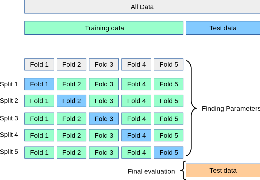
Let’s improve our fitting with k-fold cross validation

1. Break the data into a training set and test set
2. Split the training set into k subsets (or folds), holding out one subset as the test set
3. Run the learning algorithm on each combination of subsets, using the average of all of the runs to find the best fitting model parameters

For more information, see the scikit-learn docs

The cross_val_score() function will automatically partition the training set into k folds, fit the model to the subset, and return the scores for each partition.

It takes a Pipeline object, the training features, and the training labels as arguments

from sklearn.model_selection import cross_val_score

Let’s do 3-fold cross validation

Linear pipeline (baseline)

model = linear_pipe['linearregression']

# Make a linear pipeline
linear_pipe = make_pipeline(StandardScaler(), LinearRegression())

# Run the 3-fold cross validation
scores = cross_val_score(
    linear_pipe,
    X_train,
    y_train,
    cv=3,
)

# Report
print("R^2 scores = ", scores)
print("Scores mean = ", scores.mean())
print("Score std dev = ", scores.std())

R^2 scores =  [ 0.02064625 -0.84773581 -0.53652985]
Scores mean =  -0.4545398042994617
Score std dev =  0.35922474493059153

Random forest model

# Make a random forest pipeline
forest_pipe = make_pipeline(
    StandardScaler(), RandomForestRegressor(n_estimators=100, random_state=42)
)

# Run the 3-fold cross validation
scores = cross_val_score(
    forest_pipe,
    X_train,
    y_train,
    cv=3,
)

# Report
print("R^2 scores = ", scores)
print("Scores mean = ", scores.mean())
print("Score std dev = ", scores.std())

R^2 scores =  [0.5208505  0.78257711 0.66646144]
Scores mean =  0.6566296832385494
Score std dev =  0.1070753730357217

Takeaway: the random forest model is clearly more accurate

Question: Why did I choose to use 100 estimators in the RF model?

• In this case, I didn’t have a good reason
• n_estimators is a model hyperparameter
• In practice, it’s best to optimize the hyperparameters and the model parameters (via the fit() method)

This is when cross validation becomes very important

• Optimizing hyperparameters with a single train/test split means you are really optimizing based on your test set.
• If you use cross validation, a final test set will always be held in reserve to do a final evaluation.

Enter GridSearchCV

A utility function that will: - Iterate over a grid of hyperparameters - Perform k-fold cross validation - Return the parameter combination with the best overall score

More info

from sklearn.model_selection import GridSearchCV

Let’s do a search over the n_estimators parameter and the max_depth parameter:

# Create our regression pipeline
pipe = make_pipeline(StandardScaler(), RandomForestRegressor(random_state=42))
pipe

Pipeline(steps=[('standardscaler', StandardScaler()),
                ('randomforestregressor',
                 RandomForestRegressor(random_state=42))])

In a Jupyter environment, please rerun this cell to show the HTML representation or trust the notebook.
On GitHub, the HTML representation is unable to render, please try loading this page with nbviewer.org.

Make the grid of parameters to search

• NOTE: you must prepend the name of the pipeline step
• The syntax for parameter names is: “[step name]__[parameter name]”

pipe.named_steps

{'standardscaler': StandardScaler(),
 'randomforestregressor': RandomForestRegressor(random_state=42)}

model_step = "randomforestregressor"
param_grid = {
    f"{model_step}__n_estimators": [5, 10, 15, 20, 30, 50, 100, 200],
    f"{model_step}__max_depth": [2, 5, 7, 9, 13, 21, 33, 51],
}

param_grid

{'randomforestregressor__n_estimators': [5, 10, 15, 20, 30, 50, 100, 200],
 'randomforestregressor__max_depth': [2, 5, 7, 9, 13, 21, 33, 51]}

# Create the grid and use 3-fold CV
grid = GridSearchCV(pipe, param_grid, cv=3, verbose=1)

# Run the search
grid.fit(X_train, y_train)

Fitting 3 folds for each of 64 candidates, totalling 192 fits

GridSearchCV(cv=3,
             estimator=Pipeline(steps=[('standardscaler', StandardScaler()),
                                       ('randomforestregressor',
                                        RandomForestRegressor(random_state=42))]),
             param_grid={'randomforestregressor__max_depth': [2, 5, 7, 9, 13,
                                                              21, 33, 51],
                         'randomforestregressor__n_estimators': [5, 10, 15, 20,
                                                                 30, 50, 100,
                                                                 200]},
             verbose=1)

In a Jupyter environment, please rerun this cell to show the HTML representation or trust the notebook.
On GitHub, the HTML representation is unable to render, please try loading this page with nbviewer.org.

# The best estimator
grid.best_estimator_

Pipeline(steps=[('standardscaler', StandardScaler()),
                ('randomforestregressor',
                 RandomForestRegressor(max_depth=7, random_state=42))])

In a Jupyter environment, please rerun this cell to show the HTML representation or trust the notebook.
On GitHub, the HTML representation is unable to render, please try loading this page with nbviewer.org.

# The best hyper parameters
grid.best_params_

{'randomforestregressor__max_depth': 7,
 'randomforestregressor__n_estimators': 100}

Now let’s evaluate!

We’ll define a helper utility function to calculate the accuracy in terms of the mean absolute percent error

def evaluate_mape(model, X_test, y_test):
    """
    Given a model and test features/targets, print out the 
    mean absolute error and accuracy
    """
    # Make the predictions
    predictions = model.predict(X_test)

    # Absolute error
    errors = abs(predictions - y_test)
    avg_error = np.mean(errors)

    # Mean absolute percentage error
    mape = 100 * np.mean(errors / y_test)

    # Accuracy
    accuracy = 100 - mape

    print("Model Performance")
    print(f"Average Absolute Error: {avg_error:0.4f}")
    print(f"Accuracy = {accuracy:0.2f}%.")

    return accuracy

Linear model results

# Setup the pipeline
linear = make_pipeline(StandardScaler(), LinearRegression())

# Fit on train set
linear.fit(X_train, y_train)

# Evaluate on test set
evaluate_mape(linear, X_test, y_test)

Model Performance
Average Absolute Error: 0.3281
Accuracy = 94.93%.

94.92864894582036

Random forest results with default parameters

# Initialize the pipeline
base_model = make_pipeline(StandardScaler(), RandomForestRegressor(random_state=42))

# Fit the training set
base_model.fit(X_train, y_train)

# Evaluate on the test set
base_accuracy = evaluate_mape(base_model, X_test, y_test)

Model Performance
Average Absolute Error: 0.2322
Accuracy = 96.43%.

The random forest model with the optimal hyperparameters

Small improvement!

grid.best_estimator_

Pipeline(steps=[('standardscaler', StandardScaler()),
                ('randomforestregressor',
                 RandomForestRegressor(max_depth=7, random_state=42))])

In a Jupyter environment, please rerun this cell to show the HTML representation or trust the notebook.
On GitHub, the HTML representation is unable to render, please try loading this page with nbviewer.org.

# Evaluate the best random forest model
best_random = grid.best_estimator_
random_accuracy = evaluate_mape(best_random, X_test, y_test)

# What's the improvement?
improvement = 100 * (random_accuracy - base_accuracy) / base_accuracy
print(f'Improvement of {improvement:0.4f}%.')

Model Performance
Average Absolute Error: 0.2320
Accuracy = 96.43%.
Improvement of 0.0011%.

Recap

• Decision trees and random forests
• Cross validation with cross_val_score
• Optimizing hyperparameters with GridSearchCV
• Feature importances from random forests

Part 2: Modeling residential sales in Philadelphia

In this part, we’ll use a random forest model and housing data from the Office of Property Assessment to predict residential sale prices in Philadelphia

Machine learning models are increasingly common in the real estate industry

• Airbnb recommends pricing to hosts
• Trulia converts house photos to house features
• Zillow’s Zestimate

The hedonic approach to housing prices

• An econometric approach
• Deconstruct housing price to the value of each of its parts
• Captures the “price premium” consumers are willing to pay for an extra bedroom or garage

What contributes to the price of a house?

• Property characteristics, e.g, size of the lot and the number of bedrooms
• Neighborhood features based on amenities or disamenities, e.g., access to transit or exposure to crime
• Spatial component that captures the tendency of housing prices to depend on the prices of neighboring homes

Note: We’ll focus on the first two components in this analysis

Why are these kinds of models important?

• They are used widely by cities to perform property assessment valuation
  • Train a model on recent residential sales
  • Apply the model to the entire residential housing stock to produce assessments
• Biases in the algorithmic models have important consequences for city residents

Too often, these models perpetuate inequality: low-value homes are over-assessed and high-value homes are under-assessed

Philadelphia’s assessments are…not good

• City Controller analysis of property assessments: Part 1
• City Controller analysis of assessments: Part 2
• Urban Spatial paper on algorithmic fairness with a case study on modeling Philadelphia’s home values

Data from the Office of Property Assessment

Let’s download data for properties in Philadelphia that had their last sale during 2022 (the last full calendar year)

Sources: - OpenDataPhilly - Metadata

import requests

# the CARTO API url
carto_url = "https://phl.carto.com/api/v2/sql"

# Only pull 2022 sales for single family residential properties
where = "sale_date >= '2022-01-01' and sale_date <= '2022-12-31'"
where = where + " and category_code_description IN ('SINGLE FAMILY', 'Single Family')"

# Create the query
query = f"SELECT * FROM opa_properties_public WHERE {where}"

# Make the request
params = {"q": query, "format": "geojson", "where": where}
response = requests.get(carto_url, params=params)

# Make the GeoDataFrame
salesRaw = gpd.GeoDataFrame.from_features(response.json(), crs="EPSG:4326")

salesRaw.head()

	geometry	cartodb_id	assessment_date	basements	beginning_point	book_and_page	building_code	building_code_description	category_code	category_code_description	census_tract	central_air	cross_reference	date_exterior_condition	depth	exempt_building	exempt_land	exterior_condition	fireplaces	frontage	fuel	garage_spaces	garage_type	general_construction	geographic_ward	homestead_exemption	house_extension	house_number	interior_condition	location	mailing_address_1	mailing_address_2	mailing_care_of	mailing_city_state	mailing_street	mailing_zip	market_value	market_value_date	number_of_bathrooms	number_of_bedrooms	number_of_rooms	number_stories	off_street_open	other_building	owner_1	owner_2	parcel_number	parcel_shape	quality_grade	recording_date	registry_number	sale_date	sale_price	separate_utilities	sewer	site_type	state_code	street_code	street_designation	street_direction	street_name	suffix	taxable_building	taxable_land	topography	total_area	total_livable_area	type_heater	unfinished	unit	utility	view_type	year_built	year_built_estimate	zip_code	zoning	pin	building_code_new	building_code_description_new	objectid
0	POINT (-75.14337 40.00957)	1077	2022-05-24T00:00:00Z	D	415' N OF ERIE AVE	54230032	O30	ROW 2 STY MASONRY	1	SINGLE FAMILY	198	N	None	None	45.0	0.0	0.0	4	0.0	16.0	None	0.0	None	A	43	0	None	3753	4	3753 N DELHI ST	None	None	None	DELRAY BEACH FL	4899 NW 6TH STREET	33445	73800	None	1.0	3.0	NaN	2.0	1683.0	None	RJ SIMPLE SOLUTION LLC	None	432345900	E	C	2023-10-04T00:00:00Z	100N040379	2022-06-13T00:00:00Z	35000	None	None	None	FL	28040	ST	N	DELHI	None	59040.0	14760.0	F	720.0	960.0	H	None	None	None	I	1942	Y	19140	RM1	1001175031	24	ROW PORCH FRONT	394097870
1	POINT (-75.13389 40.03928)	1108	2022-05-24T00:00:00Z	H	241' N OF CHEW ST	54230133	R30	ROW B/GAR 2 STY MASONRY	1	SINGLE FAMILY	275	N	None	None	95.0	0.0	0.0	7	0.0	15.0	None	1.0	None	B	61	0	None	5732	4	5732 N 7TH ST	WALKER MICHAEL	None	None	SICKLERVILLE NJ	44 FARMHOUSE RD	08081	133400	None	1.0	3.0	NaN	2.0	1920.0	None	WALKER MICHAEL	None	612234600	E	C	2023-10-04T00:00:00Z	135N7 61	2022-08-21T00:00:00Z	21000	None	None	None	NJ	87930	ST	N	7TH	None	106720.0	26680.0	F	1425.0	1164.0	H	None	None	None	I	1925	Y	19120	RSA5	1001602509	24	ROW PORCH FRONT	394097901
2	POINT (-75.07249 40.01381)	1280	2022-05-24T00:00:00Z	D	119'11 1/2" NE	54228837	H30	SEMI/DET 2 STY MASONRY	1	SINGLE FAMILY	299	N	None	None	76.0	0.0	0.0	4	0.0	20.0	None	0.0	None	B	62	0	None	5033	4	5033 DITMAN ST	CSC INGEO	None	None	PHILADELPHIA PA	5033 DITMAN ST	19124-2230	119100	None	1.0	3.0	NaN	2.0	698.0	None	LISHANSKY MARINA	None	622444400	E	C	2023-10-02T00:00:00Z	89N17 208	2022-12-28T00:00:00Z	1	None	None	None	PA	28660	ST	None	DITMAN	None	95280.0	23820.0	F	1523.0	1190.0	B	None	None	None	I	1945	None	19124	RSA5	1001181518	32	TWIN CONVENTIONAL	394098073
3	POINT (-75.12854 40.03916)	1693	2022-05-24T00:00:00Z	None	71'8" E LAWRENCE ST	54226519	O30	ROW 2 STY MASONRY	1	SINGLE FAMILY	274	None	None	None	88.0	0.0	0.0	4	0.0	14.0	None	0.0	None	A	61	0	None	416	4	416 W GRANGE AVE	None	None	None	PHILADELPHIA PA	416 W GRANGE AVE	19120-1854	124100	None	1.0	3.0	NaN	2.0	957.0	None	WALLACE DANE	None	612061100	E	C	2023-09-25T00:00:00Z	122N2 150	2022-10-26T00:00:00Z	1	None	None	None	PA	38040	AVE	W	GRANGE	None	99280.0	24820.0	F	1241.0	1104.0	None	None	None	None	I	1953	Y	19120	RSA5	1001249126	24	ROW PORCH FRONT	394098484
4	POINT (-75.17362 39.99887)	2606	2022-05-24T00:00:00Z	D	261'4" N OF SOMERSET	54217081	O50	ROW 3 STY MASONRY	1	SINGLE FAMILY	172	N	None	None	56.0	0.0	0.0	4	0.0	16.0	None	0.0	None	B	38	0	None	2834	4	2834 N 26TH ST	NEAL KIYONNA	None	None	PHILADELPHIA PA	6007 N FRONT ST	19120	92900	None	0.0	5.0	NaN	3.0	2457.0	None	NEAL KIYONNA	None	381152100	E	C+	2023-08-28T00:00:00Z	035N230348	2022-05-11T00:00:00Z	1	None	None	None	PA	88300	ST	N	26TH	None	74320.0	18580.0	F	896.0	1636.0	H	None	None	None	I	1940	Y	19132	RSA5	1001643492	24	ROW PORCH FRONT	394099946

len(salesRaw)

24457

The OPA is messy

Lots of missing data.

We can use the missingno package to visualize the missing data easily.

import missingno as msno

# We'll visualize the first half of columns
# and then the second half
ncol = len(salesRaw.columns)

fields1 = salesRaw.columns[:ncol//2]
fields2 = salesRaw.columns[ncol//2:]

ncol

80

# The first half of columns
msno.bar(salesRaw[fields1]);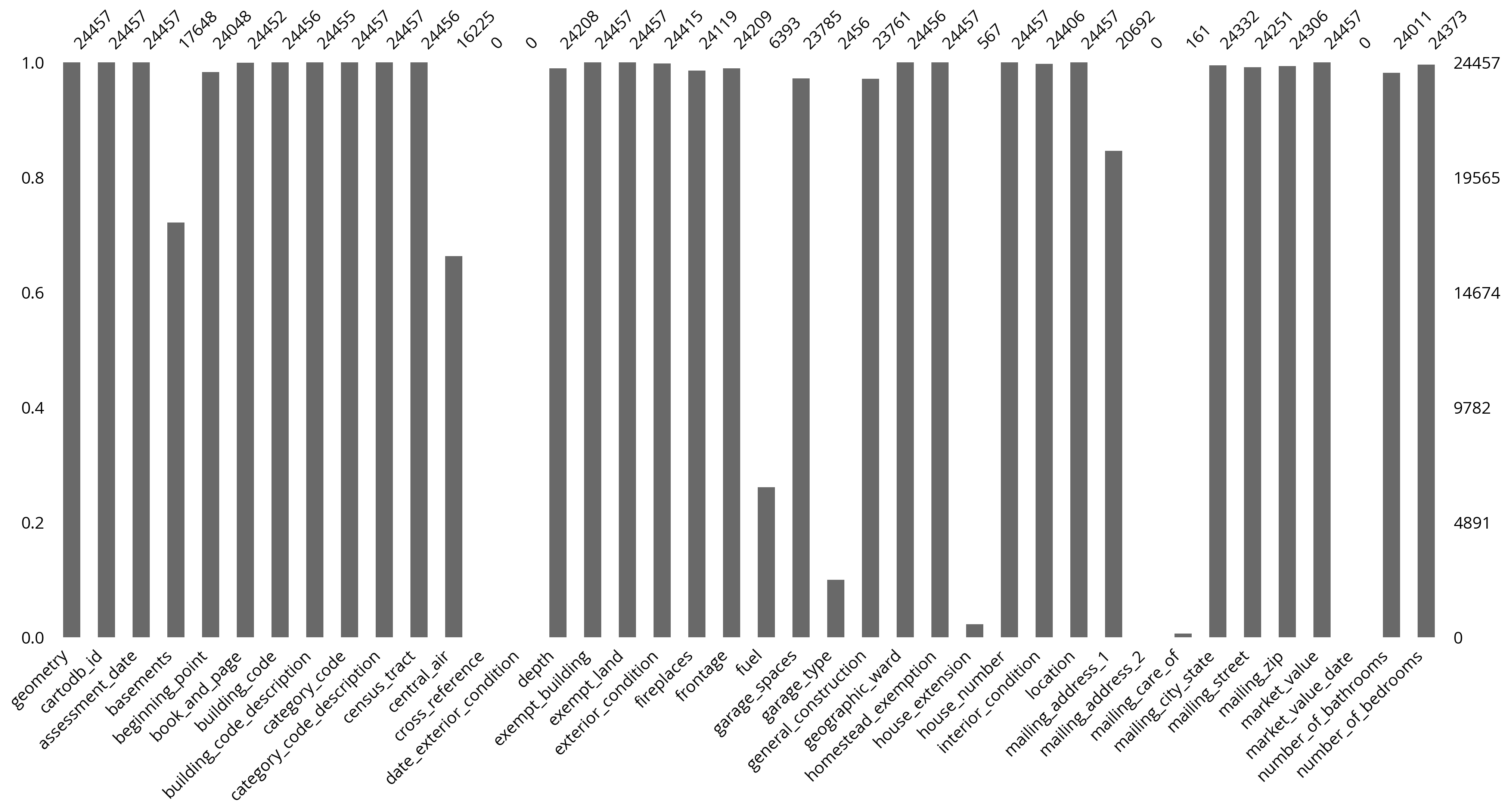

# The second half of columns
msno.bar(salesRaw[fields2]);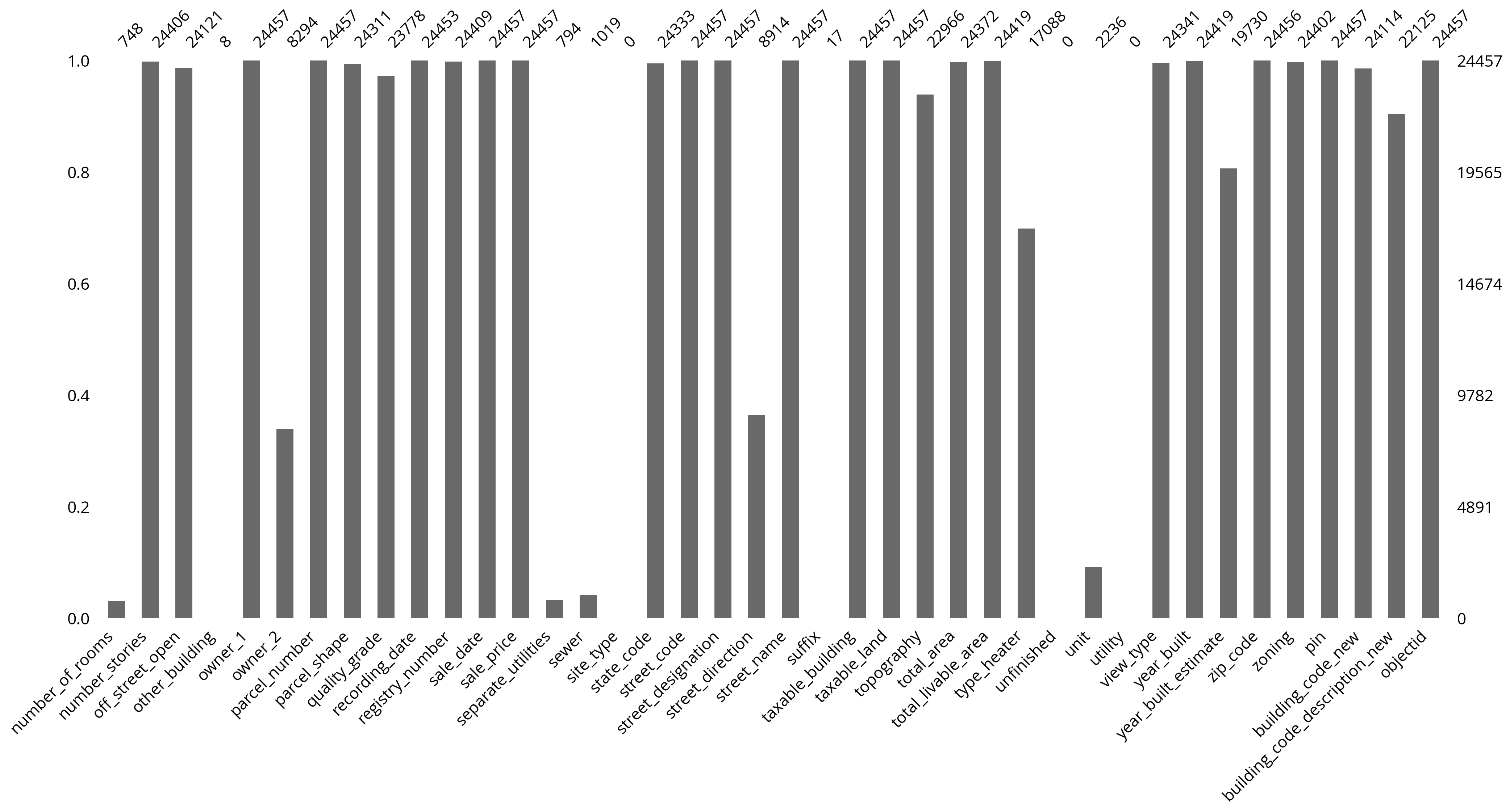

# The feature columns we want to use
cols = [
    "sale_price",
    "total_livable_area",
    "total_area",
    "garage_spaces",
    "fireplaces",
    "number_of_bathrooms",
    "number_of_bedrooms",
    "number_stories",
    "exterior_condition",
    "zip_code",
]

# Trim to these columns and remove NaNs
sales = salesRaw[cols].dropna()

# Trim zip code to only the first five digits
sales['zip_code'] = sales['zip_code'].astype(str).str.slice(0, 5)

len(sales)

23479

# Trim very low and very high sales
valid = (sales['sale_price'] > 3000) & (sales['sale_price'] < 1e6)
sales = sales.loc[valid]

len(sales)

17684

Let’s focus on numerical features only first

# Split the data 70/30
train_set, test_set = train_test_split(sales, test_size=0.3, random_state=42)

# the target labels: log of sale price
y_train = np.log(train_set["sale_price"])
y_test = np.log(test_set["sale_price"])

# The features
feature_cols = [
    "total_livable_area",
    "total_area",
    "garage_spaces",
    "fireplaces",
    "number_of_bathrooms",
    "number_of_bedrooms",
    "number_stories",
]
X_train = train_set[feature_cols].values
X_test = test_set[feature_cols].values

# Make a random forest pipeline
forest = make_pipeline(
    StandardScaler(), RandomForestRegressor(n_estimators=100, random_state=42)
)

# Run the 10-fold cross validation
scores = cross_val_score(
    forest,
    X_train,
    y_train,
    cv=10,
)

# Report
print("R^2 scores = ", scores)
print("Scores mean = ", scores.mean())
print("Score std dev = ", scores.std())

R^2 scores =  [0.31590527 0.24439146 0.34501458 0.29939277 0.30929715 0.32289248
 0.429871   0.2990362  0.32022697 0.33481283]
Scores mean =  0.32208407045926973
Score std dev =  0.04426497345382467

# Fit on the training data
forest.fit(X_train, y_train)

# What's the test score?
forest.score(X_test, y_test)

0.3114781077490535

Which variables were most important?

# Extract the regressor from the pipeline
regressor = forest["randomforestregressor"]

# Create the data frame of importances
importance = pd.DataFrame(
    {
     "Feature": feature_cols, 
     "Importance": regressor.feature_importances_
    }
).sort_values(by="Importance")

importance.hvplot.barh(x="Feature", y="Importance")

Takeaway: Number of bathrooms and area-based features still important

To be continued next lecture…