Week 3B: Intro to Geospatial Data Analysis with GeoPandas

Section 401
Sep 20, 2023

Housekeeping

Homework #1 due on Monday (9/25)
Homework #2 will be assigned same day
Choose a dataset to visualize and explore
- OpenDataPhilly or one your choosing
- Email me if you want to analyze one that’s not on OpenDataPhilly

Agenda for today

Introduction to GeoPandas and vector data
Spatial relationships and joins

Note

We’ll continue geospatial analysis next week, with: - Visualization for geospatial data - Demo: 311 requests by neighborhood in Philadelphia - Exercise: Property assessments by neighborhood

# Let's setup the imports we'll need first

import altair as alt
import numpy as np
import pandas as pd
import seaborn as sns
from matplotlib import pyplot as plt

%matplotlib inline

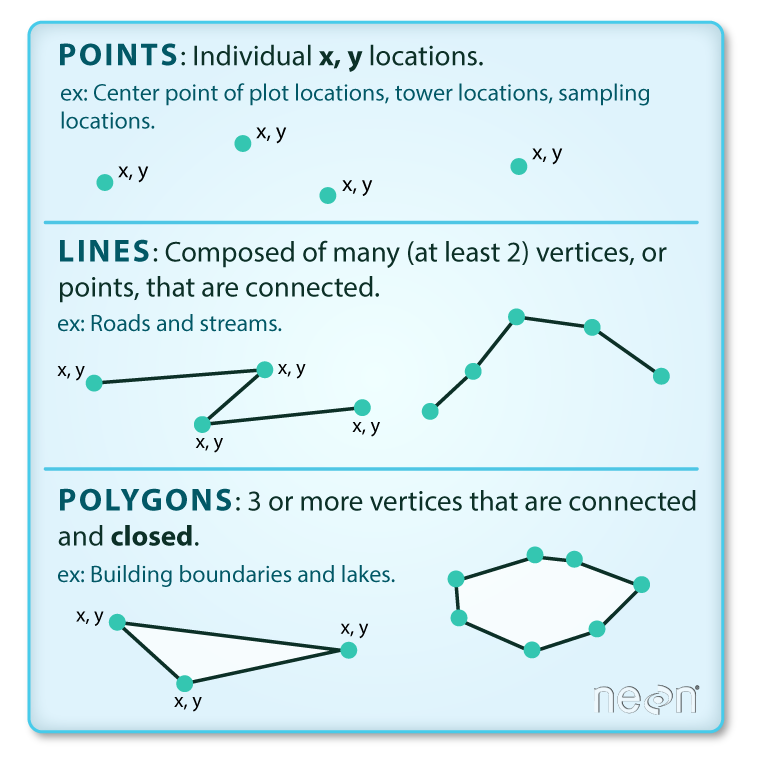
Part 1: Vector geospatial data in Python

Vector refers to discrete geometric entities
The Open Geospatial Consortium has standardized a set of simple features
Includes points, lines, and polygons

Source

A couple of terminology notes

A feature refers to both the geometry and attributes of specific piece of vector data
A feature collection is a list, or collection, of features

Both terms are very common in Python geospatial software.

Common formats for vector datasets

1. A shapefile

Actually several files with the same common prefix.

Mandatory files:

.shp: the file containing the geometries
.shx: the file that indexes the geometry
.dbf: tabular data format storing the attributes for each geometry

And many optional files for documentation, projection information, etc.

Let’s take a look at an example shapefile:

We’ll use the %ls command to list out all of the files in an example shapefile in the data/ folder

%ls "data/ne_110m_admin_0_countries/"

ne_110m_admin_0_countries.cpg  ne_110m_admin_0_countries.shp
ne_110m_admin_0_countries.dbf  ne_110m_admin_0_countries.shx
ne_110m_admin_0_countries.prj

2. The GeoJSON file

Stores simple features in a JSON format
Arose due to the prevalence of the JSON format, especially on the web

Additional GeoJSON resources

GitHub lets you view GeoJSON files natively. See Philadelphia ZIP Codes in the data/ folder of this week’s repo.
http://geojson.io provides interactive creation and viewing of small GeoJSON files

Analyzing vector data with GeoPandas

geopandas provides a simple, intuitive for the main types of geospatial vector file formats

# The import statement
import geopandas as gpd

Example: Let’s load a shape file of countries in the world…

Source: Natural Earth Data

We can use the read_file() function to read shapefiles and GeoJSON files.

# Read the shape file, giving the name of the directory
countries = gpd.read_file("./data/ne_110m_admin_0_countries")

countries.head()

	iso_a3	name	continent	pop_est	gdp_md_est	geometry
0	AFG	Afghanistan	Asia	34124811.0	64080.0	POLYGON ((61.21082 35.65007, 62.23065 35.27066...
1	AGO	Angola	Africa	29310273.0	189000.0	MULTIPOLYGON (((23.90415 -11.72228, 24.07991 -...
2	ALB	Albania	Europe	3047987.0	33900.0	POLYGON ((21.02004 40.84273, 20.99999 40.58000...
3	ARE	United Arab Emirates	Asia	6072475.0	667200.0	POLYGON ((51.57952 24.24550, 51.75744 24.29407...
4	ARG	Argentina	South America	44293293.0	879400.0	MULTIPOLYGON (((-66.95992 -54.89681, -67.56244...

type(countries)

geopandas.geodataframe.GeoDataFrame

What’s a `GeoDataFrame`?

Just like a DataFrame but with a new, special geometry column:

Print out the first 10 entires of the “geometry” column:

countries["geometry"].head(n=10)

0    POLYGON ((61.21082 35.65007, 62.23065 35.27066...
1    MULTIPOLYGON (((23.90415 -11.72228, 24.07991 -...
2    POLYGON ((21.02004 40.84273, 20.99999 40.58000...
3    POLYGON ((51.57952 24.24550, 51.75744 24.29407...
4    MULTIPOLYGON (((-66.95992 -54.89681, -67.56244...
5    POLYGON ((43.58275 41.09214, 44.97248 41.24813...
6    MULTIPOLYGON (((-59.57209 -80.04018, -59.86585...
7    POLYGON ((68.93500 -48.62500, 69.58000 -48.940...
8    MULTIPOLYGON (((145.39798 -40.79255, 146.36412...
9    POLYGON ((16.97967 48.12350, 16.90375 47.71487...
Name: geometry, dtype: geometry

Take a look at the first geometry polygon by using the .iloc[] selector:

countries['geometry'].iloc[0]

We can still leverage the power of `pandas`…

Calculate the total world population:

countries["pop_est"].sum() / 1e9  # In billions

7.383089462

Calculate the total population on each continent:

grouped = countries.groupby("continent")

grouped

<pandas.core.groupby.generic.DataFrameGroupBy object at 0x17f287b80>

Remember

The groupby() function does not return a DataFrame — you need to call sum(), mean() etc, or apply() a function to get your desired result!

Access the “pop_est” column from the groupby variable (“grouped”) and then call the .sum() function to calculate our desired statistic:

pop_by_continent = grouped["pop_est"].sum()

pop_by_continent

continent
Africa                     1.219176e+09
Antarctica                 4.050000e+03
Asia                       4.389145e+09
Europe                     7.463985e+08
North America              5.730421e+08
Oceania                    3.678284e+07
Seven seas (open ocean)    1.400000e+02
South America              4.185407e+08
Name: pop_est, dtype: float64

# Sort values
pop_by_continent.sort_values(ascending=False, inplace=True)

# Output sorted values from cell
pop_by_continent / 1e9

continent
Asia                       4.389145e+00
Africa                     1.219176e+00
Europe                     7.463985e-01
North America              5.730421e-01
South America              4.185407e-01
Oceania                    3.678284e-02
Antarctica                 4.050000e-06
Seven seas (open ocean)    1.400000e-07
Name: pop_est, dtype: float64

Filter the data frame based on a boolean selection:

# Is the country name USA?
is_USA = countries["name"] == "United States of America"

is_USA

0      False
1      False
2      False
3      False
4      False
       ...  
172    False
173    False
174    False
175    False
176    False
Name: name, Length: 177, dtype: bool

# Get the row with USA
USA = countries.loc[is_USA]

USA

	iso_a3	name	continent	pop_est	gdp_md_est	geometry
168	USA	United States of America	North America	326625791.0	18560000.0	MULTIPOLYGON (((-122.84000 49.00000, -120.0000...

USA.squeeze().geometry

Reminder: the squeeze() function

The squeeze() function does just one it sounds like: if you have a DataFrame with only one row, it will “squeeze” the row dimension by removing it, returning just a Series object:

# Squeeze
USA = USA.squeeze()

# Print out the types
print("The type of USA is: ", type(USA))

# Output
USA

The type of USA is:  <class 'pandas.core.series.Series'>

iso_a3                                                      USA
name                                   United States of America
continent                                         North America
pop_est                                             326625791.0
gdp_md_est                                           18560000.0
geometry      MULTIPOLYGON (((-122.84000000000005 49.0000000...
Name: 168, dtype: object

The simple features (Lines, Points, Polygons) are implemented by the shapely library

USA

iso_a3                                                      USA
name                                   United States of America
continent                                         North America
pop_est                                             326625791.0
gdp_md_est                                           18560000.0
geometry      MULTIPOLYGON (((-122.84000000000005 49.0000000...
Name: 168, dtype: object

type(USA.geometry)

shapely.geometry.multipolygon.MultiPolygon

JupyterLab renders shapely geometries automatically:

# a mini USA
USA.geometry

How does `geopandas` handle coordinate systems and map projections?

A coordinate reference system (CRS) relates the position of a geometry object on the spherical earth to its two-dimensional coordinates.

A GeoDataFrame or GeoSeries has a .crs attribute which specifies the coordinate reference system.

countries.crs

<Geographic 2D CRS: EPSG:4326>
Name: WGS 84
Axis Info [ellipsoidal]:
- Lat[north]: Geodetic latitude (degree)
- Lon[east]: Geodetic longitude (degree)
Area of Use:
- name: World.
- bounds: (-180.0, -90.0, 180.0, 90.0)
Datum: World Geodetic System 1984 ensemble
- Ellipsoid: WGS 84
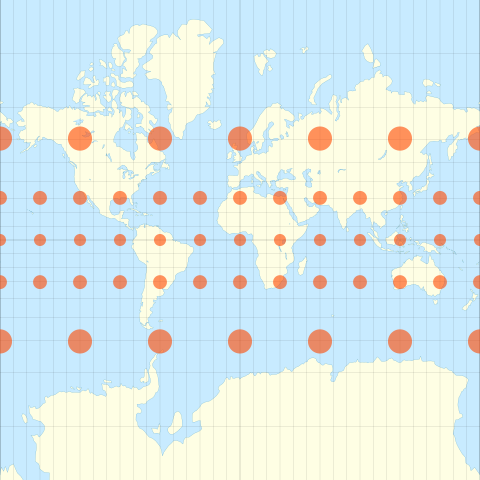
- Prime Meridian: Greenwich

The EPSG=4326 CRS

EPSG 4326 is known as WGS 84 where x and y are longitude and latitude.
It is is the default coordinate system for GPS systems.
It’s also known as Plate Carrée or equirectangular

How to plot all of the geometries at once?

Use the plot() function to get a quick and dirty plot of all of the geometry features.

Note: the plot() returns the current maplotlib axes, allowing you to format the chart after plotting.

# Create a figure and axes
fig, ax = plt.subplots(figsize=(10, 6))

# Plot the countries on our axes
ax = countries.plot(ax=ax, facecolor="none", edgecolor="black")

# Add a title
ax.set_title("Equirectangular Projection");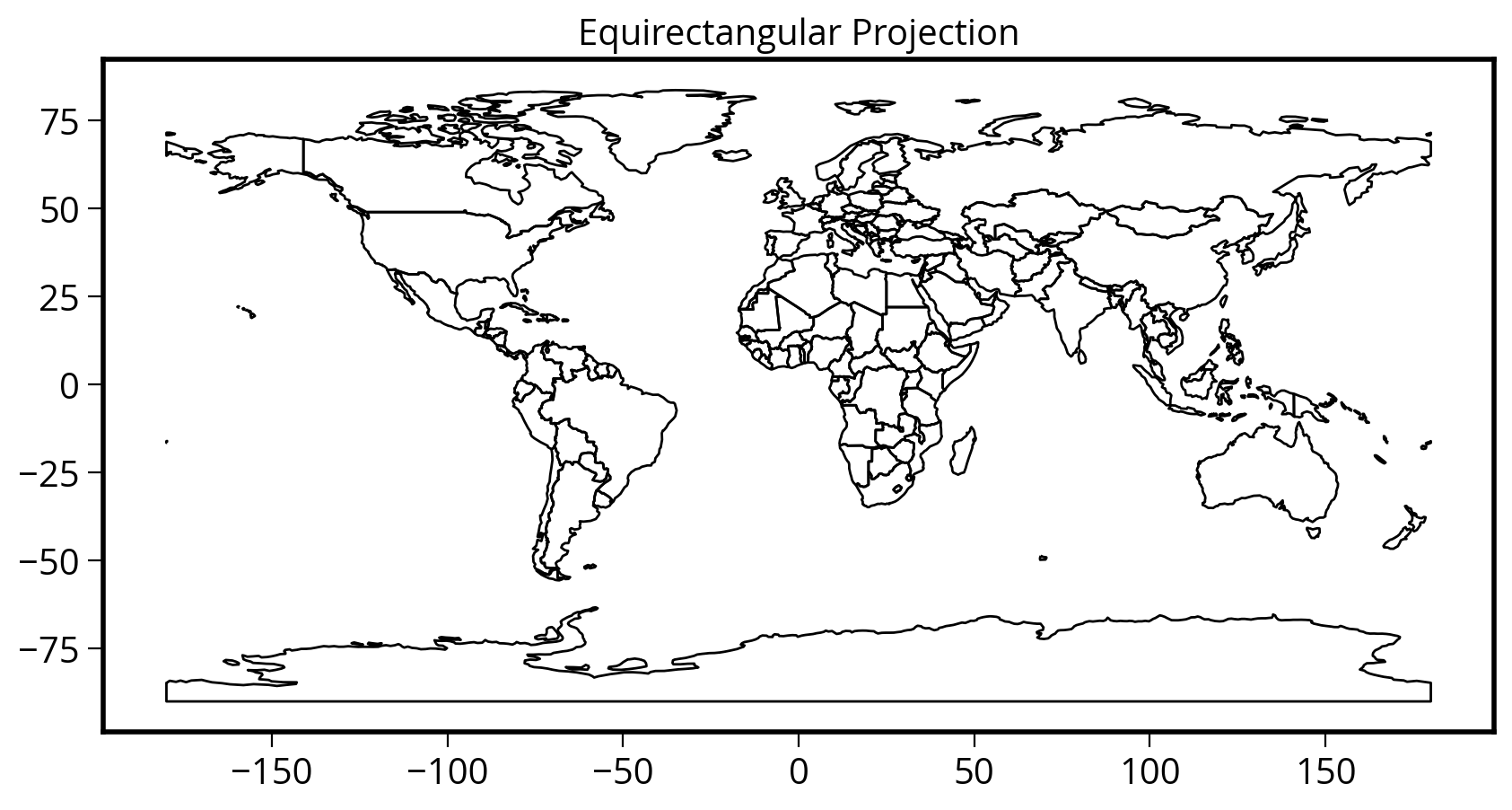

Can we convert to other coordinate systems?

Use the df.to_crs() function! The most well-known projections can be specified by their EPSG code.

Geopandas documentation on re-projecting: Managing Projections

Let’s convert to the Mercator projection

EPSG code: 3395

# Remove Antartica, as the Mercator projection
# cannot deal with the poles
no_antarctica = countries.loc[(countries["name"] != "Antarctica")]

# Two ways to specify the EPSG code
countries_mercator = no_antarctica.to_crs(epsg=3395)

# Alternatively:
# countries_mercator = no_antartica.to_crs("EPSG:3395")

countries_mercator.head()

	iso_a3	name	continent	pop_est	gdp_md_est	geometry
0	AFG	Afghanistan	Asia	34124811.0	64080.0	POLYGON ((6813956.990 4227673.562, 6927484.435...
1	AGO	Angola	Africa	29310273.0	189000.0	MULTIPOLYGON (((2660998.216 -1305442.810, 2680...
2	ALB	Albania	Europe	3047987.0	33900.0	POLYGON ((2339940.185 4961221.199, 2337708.178...
3	ARE	United Arab Emirates	Asia	6072475.0	667200.0	POLYGON ((5741805.754 2765811.385, 5761611.935...
4	ARG	Argentina	South America	44293293.0	879400.0	MULTIPOLYGON (((-7453944.198 -7306880.704, -75...

Tip

Take a look at the values in the “geometry” column above. The magnitude of the coordinates changed! This is a quick and easy way to tell if the re-projection worked properly!

Now let’s plot it!

The easy way…with geopandas built-in plot() function

# Initialize the figure and axes
fig, ax = plt.subplots(figsize=(10, 6))

# Use built-in plot() of the GeoDataFrame
ax = countries_mercator.plot(ax=ax, facecolor="none", edgecolor="black")

# Add a title
ax.set_title("Mercator Projection");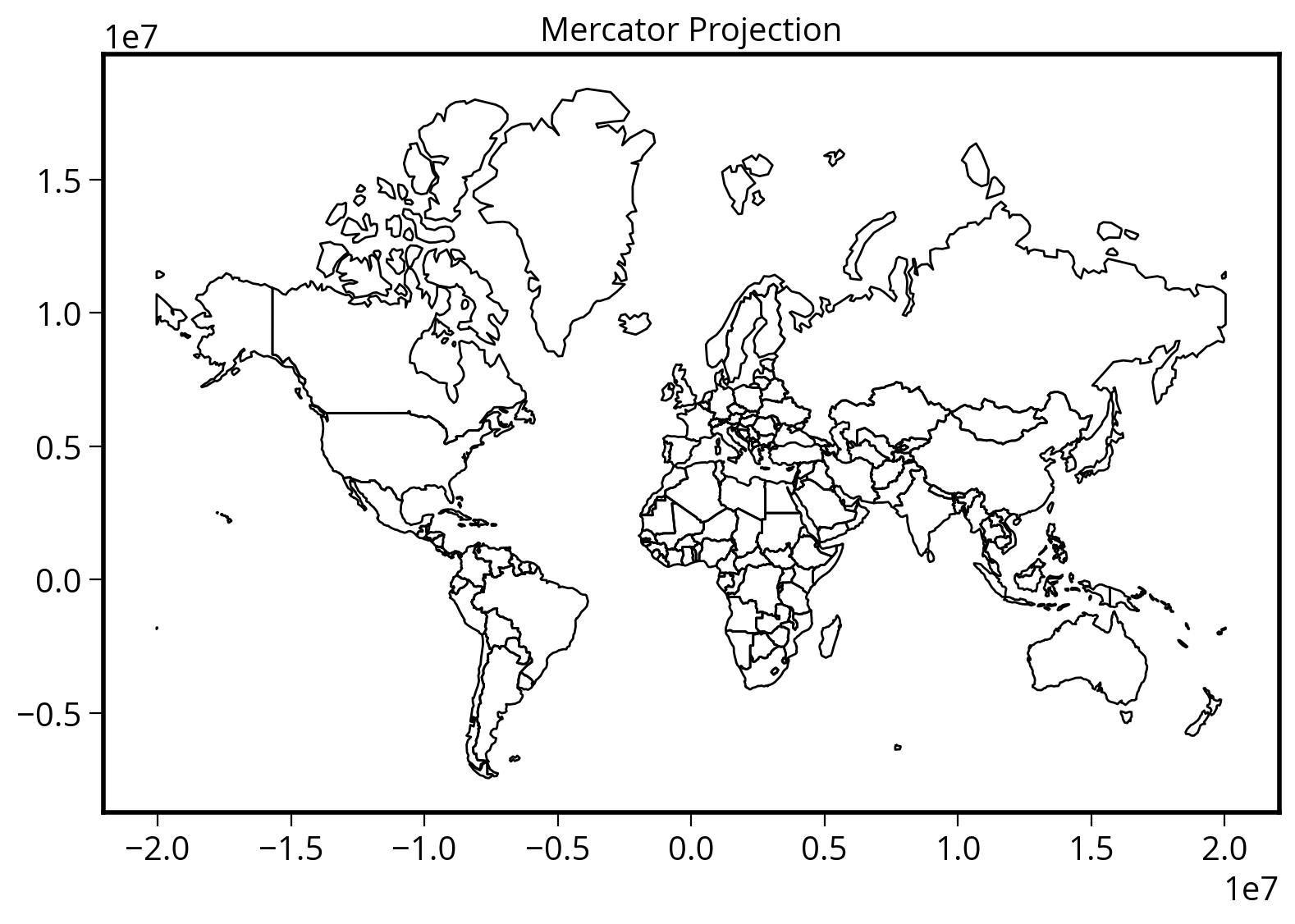

Which one is your favorite?

Source: xkcd

Tip: Choosing the right CRS

For city-based data, the Web Mercator CRS (EPSG=3857) is best. This CRS became popular after Google Maps adopted it.
You can also use a CRS specific to individual states, e.g., the PA State Plane EPSG=2272 is a good option for Philadelphia

Let’s load the city limits for Philadelphia

We’ll use the provided City_Limits shape file in the data/ folder

city_limits = gpd.read_file("./data/City_Limits")

city_limits

	OBJECTID	Shape__Are	Shape__Len	geometry
0	1	0.038911	1.259687	POLYGON ((-75.01497 40.13793, -75.01456 40.137...

What’s the CRS?

Use the .crs attribute to find out!

city_limits.crs

<Geographic 2D CRS: EPSG:4326>
Name: WGS 84
Axis Info [ellipsoidal]:
- Lat[north]: Geodetic latitude (degree)
- Lon[east]: Geodetic longitude (degree)
Area of Use:
- name: World.
- bounds: (-180.0, -90.0, 180.0, 90.0)
Datum: World Geodetic System 1984 ensemble
- Ellipsoid: WGS 84
- Prime Meridian: Greenwich

Plot it with the EPSG=4326 CRS:

# Create our figure and axes
fig, ax = plt.subplots(figsize=(5, 5))

# Plot
city_limits.plot(ax=ax, facecolor="none", edgecolor="black")

# Format
ax.set_title("Equirectangular")
ax.set_axis_off()  # This will remove the axes completely
ax.set_aspect("equal")  # This forces an equal aspect ratio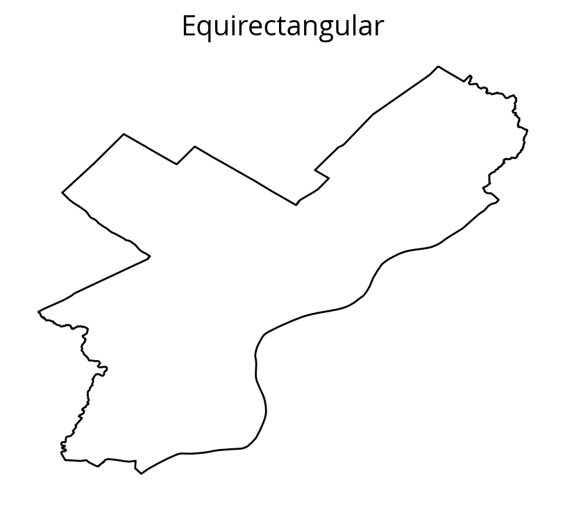

This is not what Philadelphia looks like..

Let’s try EPSG=3857 instead:

# Create the figure
fig, ax = plt.subplots(figsize=(5, 5))

# Convert to EPSG:3857
city_limits_3857 = city_limits.to_crs(epsg=3857)

# Plot and format
city_limits_3857.plot(ax=ax, facecolor="none", edgecolor="black")

ax.set_title("Web Mercator")
ax.set_axis_off()
ax.set_aspect("equal");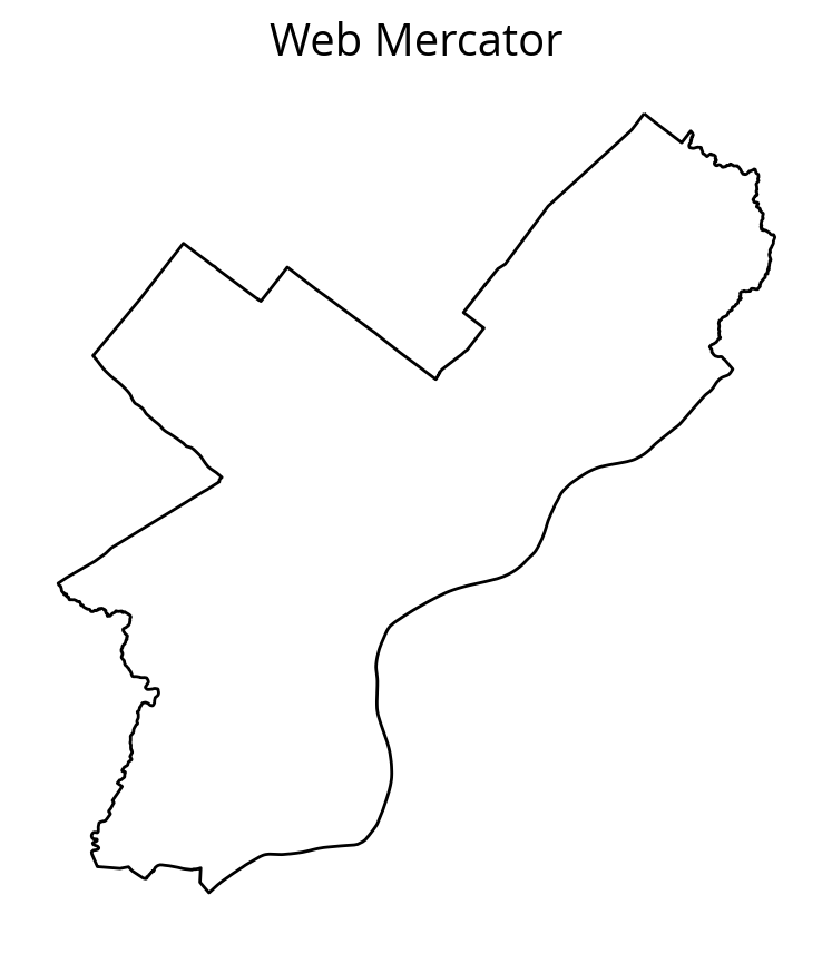

Important

The equirectangular CRS (EPSG=4326) is often used by default and will make cities appear wider and flatter than they really are.

Saving GeoDataFrames

Use the to_file() function and specify the driver.

# ESRI shape file
city_limits_3857.to_file("./data/city_limits_3857", driver="Shapefile")

# GeoJSON is also an option
city_limits_3857.to_file("./data/city_limits_3857.geojson", driver="GeoJSON")

How about as a CSV file?

Yes, but reading requires more work…

# save a csv file
city_limits_3857.to_csv("./data/city_limits_3857.csv", index=False)

df = pd.read_csv("./data/city_limits_3857.csv")

df.head()

	OBJECTID	Shape__Are	Shape__Len	geometry
0	1	0.038911	1.259687	POLYGON ((-8350627.97509646 4886006.88680784, ...

Looks similar…

But, the “geometry” column is just stored as a string…it’s not a shapely Polygon

df.geometry

0    POLYGON ((-8350627.97509646 4886006.88680784, ...
Name: geometry, dtype: object

Use `shapely` to parse the string version of the polygons

from shapely import wkt

# wkt.loads will convert from string to Polygon object
df["geometry"] = df["geometry"].apply(wkt.loads)

df.geometry.iloc[0]

Success!

Converting from a DataFrame to a GeoDataFrame

We can initialize the GeoDataFrame directly from a DataFrame but we need to specify two things:

The name of the “geometry” column
The CRS of the “geometry” column

Watch out!

The CRS that you specify when you create the GeoDataFrame must match the CRS of the data. It is not the CRS that you wish the data was in. If you would like to convert to a different CRS, you’ll need to call the .to_crs() after creating your GeoDataFrame.

In this case, the geometry column was saved in Web Mercator EPSG=3857

# Make specifying the name of the geometry column and CRS
gdf = gpd.GeoDataFrame(df, geometry="geometry", crs="EPSG:3857")

# Now plot
fig, ax = plt.subplots(figsize=(5, 5))
ax = gdf.plot(ax=ax, facecolor="none", edgecolor="black")
ax.set_axis_off()
ax.set_aspect("equal")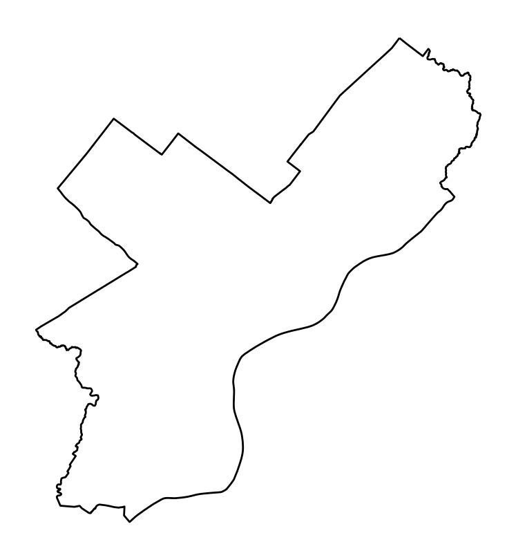

Let’s convert back to 4326 and plot

The tilt should be a bit more obvious now…

ax = gdf.to_crs(epsg=4326).plot(facecolor="none", edgecolor="black")

ax.set_axis_off()
ax.set_aspect("equal")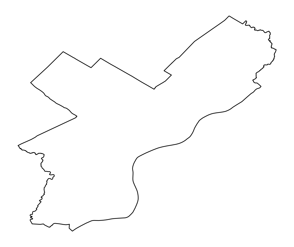

Note

I didn’t use plt.subplots() here to create a figure/axes – I let geopandas automatically make one
I’ve chained together the to_crs() and .plot() functions in one line
The .plot() function returns the axes object that geopandas used to plot — this lets you customizes the axes after plotting

So, when should you use GeoPandas?

For exploratory data analysis and visualization, including in Jupyter notebooks
Pre-processing data to be fed into a desktop GIS program
For compact, readable, and reproducible code
If you’re comfortable with Pandas and/or R data frames.

When it may not be the best tool:

For polished multilayer map creation — one option is to use a desktop GIS like QGIS.
If you need very high performance — geopandas can be slow compared to other GIS software.

Part 2: Spatial Relationships and Joins

Let’s explore joins and merges between GeoDataFrames based on geospatial relationships…

# Load some cities data from the data/ folder
cities = gpd.read_file("./data/ne_110m_populated_places")

cities

	name	geometry
0	Vatican City	POINT (12.45339 41.90328)
1	San Marino	POINT (12.44177 43.93610)
2	Vaduz	POINT (9.51667 47.13372)
3	Lobamba	POINT (31.20000 -26.46667)
4	Luxembourg	POINT (6.13000 49.61166)
...	...	...
238	Rio de Janeiro	POINT (-43.22697 -22.92308)
239	São Paulo	POINT (-46.62697 -23.55673)
240	Sydney	POINT (151.18323 -33.91807)
241	Singapore	POINT (103.85387 1.29498)
242	Hong Kong	POINT (114.18306 22.30693)

243 rows × 2 columns

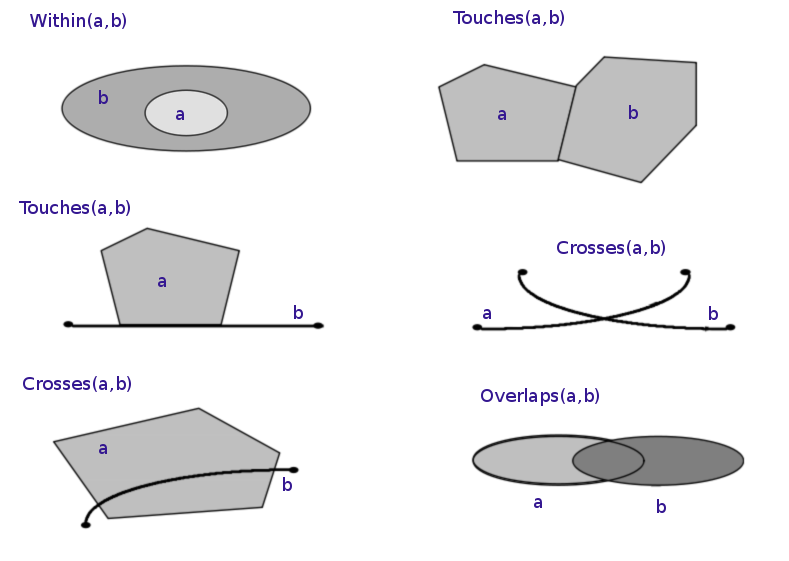
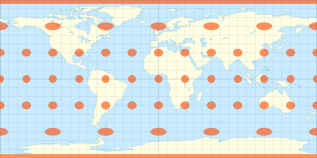
(Image by Krauss, CC BY-SA 3.0)

All of these operations are available as functions of a GeoDataFrame.

A quick example

What country is New York in?

Spoiler: the USA

# Select the Point representing New York City
new_york = cities.loc[cities["name"] == "New York"].geometry.squeeze()

new_york

type(new_york)

shapely.geometry.point.Point

countries.contains(new_york)

0      False
1      False
2      False
3      False
4      False
       ...  
172    False
173    False
174    False
175    False
176    False
Length: 177, dtype: bool

# Find the country that contains New York
countries.loc[countries.contains(new_york)]

	iso_a3	name	continent	pop_est	gdp_md_est	geometry
168	USA	United States of America	North America	326625791.0	18560000.0	MULTIPOLYGON (((-122.84000 49.00000, -120.0000...

# Get the geometry column of the country containing NYC
USA = countries.loc[countries.contains(new_york)].squeeze().geometry
USA

Note

The .loc[] function can take the index selector as the first argument, and the name of a column as a second argument (separated by a comma)

type(USA)

shapely.geometry.multipolygon.MultiPolygon

# Is New York within the USA?
new_york.within(USA)

True

USA

References

The different functions for checking spatial relationships:

equals
contains
crosses
disjoint
intersects
overlaps
touches
within
covers

See the shapely documentation for an overview of these methods.

1. The spatial join: `sjoin()`

SPATIAL JOIN = merging attributes from two geometry layers based on their spatial relationship

Different parts of this operations:

The GeoDataFrame to which we want add information
The GeoDataFrame that contains the information we want to add
The spatial relationship we want to use to match both datasets (intersects, contains, within)
The type of join: left or inner join

In this case, we want to join the cities dataframe, containing Point geometries, with the information of the countries dataframe, containing Polygon geometries.

To match cities with countries, we’ll use the within spatial relationship.

The geopandas.sjoin() function performs this operation:

joined = gpd.sjoin(
    cities,
    countries,
    predicate="within",
    how="left",
    lsuffix="city",
    rsuffix="country",
)

joined.head()

	name_city	geometry	index_country	iso_a3	name_country	continent	pop_est	gdp_md_est
0	Vatican City	POINT (12.45339 41.90328)	79.0	ITA	Italy	Europe	62137802.0	2221000.0
1	San Marino	POINT (12.44177 43.93610)	79.0	ITA	Italy	Europe	62137802.0	2221000.0
2	Vaduz	POINT (9.51667 47.13372)	9.0	AUT	Austria	Europe	8754413.0	416600.0
3	Lobamba	POINT (31.20000 -26.46667)	152.0	SWZ	Swaziland	Africa	1467152.0	11060.0
4	Luxembourg	POINT (6.13000 49.61166)	97.0	LUX	Luxembourg	Europe	594130.0	58740.0

As we can see above, the attributes of the cities (left) and countries (right) have been merged based on whether the city is inside the country.

Let’s select cities in Italy only:

cities_in_italy = joined.loc[joined["name_country"] == "Italy"]
cities_in_italy

	name_city	geometry	index_country	iso_a3	name_country	continent	pop_est	gdp_md_est
0	Vatican City	POINT (12.45339 41.90328)	79.0	ITA	Italy	Europe	62137802.0	2221000.0
1	San Marino	POINT (12.44177 43.93610)	79.0	ITA	Italy	Europe	62137802.0	2221000.0
226	Rome	POINT (12.48131 41.89790)	79.0	ITA	Italy	Europe	62137802.0	2221000.0

# Extract Italy
italy = countries.loc[countries["name"] == "Italy"]

# Plot
fig, ax = plt.subplots(figsize=(8, 8))
italy.plot(ax=ax, facecolor="none", edgecolor="black")
ax.set_axis_off()
ax.set_aspect("equal")

# Plot the first city in the joined data frame (Vatican City)
# Use the same axes by passing in the ax=ax keyword
ax = cities_in_italy.plot(ax=ax, color="red")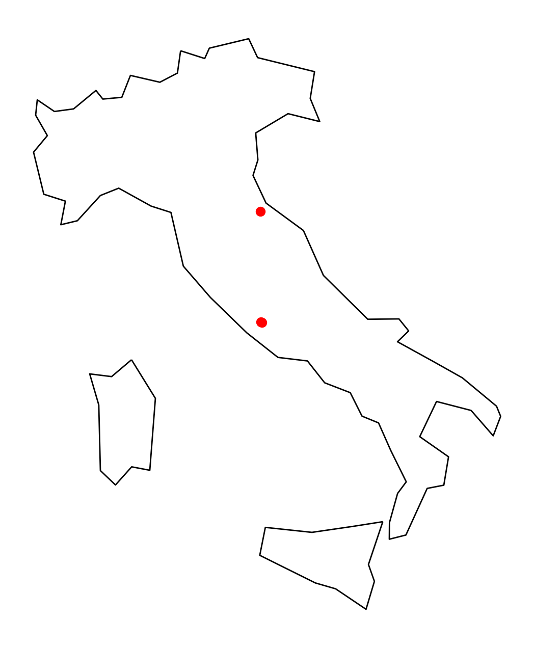

2. Spatial overlay operation: `overlay()`

We can also perform the “join” operation on the geometries rather than just combining attributes.

The overlay() function combines geometries, e.g. by taking the intersection of the geometries.

Select all countries in Africa:

africa = countries.loc[countries["continent"] == "Africa"]

africa.head()

	iso_a3	name	continent	pop_est	gdp_md_est	geometry
1	AGO	Angola	Africa	29310273.0	189000.0	MULTIPOLYGON (((23.90415 -11.72228, 24.07991 -...
11	BDI	Burundi	Africa	11466756.0	7892.0	POLYGON ((29.34000 -4.49998, 29.27638 -3.29391...
13	BEN	Benin	Africa	11038805.0	24310.0	POLYGON ((2.69170 6.25882, 1.86524 6.14216, 1....
14	BFA	Burkina Faso	Africa	20107509.0	32990.0	POLYGON ((2.15447 11.94015, 1.93599 11.64115, ...
25	BWA	Botswana	Africa	2214858.0	35900.0	POLYGON ((29.43219 -22.09131, 28.01724 -22.827...

What is the CRS?

africa.crs

<Geographic 2D CRS: EPSG:4326>
Name: WGS 84
Axis Info [ellipsoidal]:
- Lat[north]: Geodetic latitude (degree)
- Lon[east]: Geodetic longitude (degree)
Area of Use:
- name: World.
- bounds: (-180.0, -90.0, 180.0, 90.0)
Datum: World Geodetic System 1984 ensemble
- Ellipsoid: WGS 84
- Prime Meridian: Greenwich

# Let's transform to a CRS that uses meters
# instead of degrees (EPSG=3857)
africa = africa.to_crs(epsg=3857)

africa.crs

<Projected CRS: EPSG:3857>
Name: WGS 84 / Pseudo-Mercator
Axis Info [cartesian]:
- X[east]: Easting (metre)
- Y[north]: Northing (metre)
Area of Use:
- name: World between 85.06°S and 85.06°N.
- bounds: (-180.0, -85.06, 180.0, 85.06)
Coordinate Operation:
- name: Popular Visualisation Pseudo-Mercator
- method: Popular Visualisation Pseudo Mercator
Datum: World Geodetic System 1984 ensemble
- Ellipsoid: WGS 84
- Prime Meridian: Greenwich

Plot it:

fig, ax = plt.subplots(figsize=(8, 8))

africa.plot(ax=ax, facecolor="#b9f2b1")

ax.set_axis_off()
ax.set_aspect("equal")

# Important CRS needs to match!
cities_3857 = cities.to_crs(epsg=3857)

# Create a copy of the GeoDataFrame
buffered_cities = cities_3857.copy()

# Add a buffer region of 250 km around all cities
buffered_cities["geometry"] = buffered_cities.buffer(250e3)

Plot the difference of the two geometries

fig, ax = plt.subplots(figsize=(8, 8))

# Calculate the difference of the geometry sets
diff = gpd.overlay(
    africa,
    buffered_cities,
    how="difference",
)

# Plot
diff.plot(facecolor="#b9f2b1", ax=ax)
ax.set_axis_off()
ax.set_aspect("equal")

/Users/nhand/mambaforge/envs/musa-550-fall-2023/lib/python3.10/site-packages/shapely/constructive.py:181: RuntimeWarning: invalid value encountered in buffer
  return lib.buffer(
/Users/nhand/mambaforge/envs/musa-550-fall-2023/lib/python3.10/site-packages/shapely/set_operations.py:77: RuntimeWarning: invalid value encountered in difference
  return lib.difference(a, b, **kwargs)

# Data attributes are the same as the first data frame (africa)
# with an updated geometry column
diff.head()

	iso_a3	name	continent	pop_est	gdp_md_est	geometry
0	AGO	Angola	Africa	29310273.0	189000.0	MULTIPOLYGON (((2673464.087 -1449571.330, 2441...
1	BEN	Benin	Africa	11038805.0	24310.0	POLYGON ((100138.898 1231805.081, 138422.412 1...
2	BFA	Burkina Faso	Africa	20107509.0	32990.0	MULTIPOLYGON (((100138.898 1231805.081, 26368....
3	BWA	Botswana	Africa	2214858.0	35900.0	POLYGON ((3065120.801 -2659823.621, 3061281.52...
4	CAF	Central African Rep.	Africa	5625118.0	3206.0	POLYGON ((1792937.514 836963.765, 1813457.017 ...

Plot the intersection of the two geometries

fig, ax = plt.subplots(figsize=(8, 8))

# The intersection of the geometry sets
intersection = gpd.overlay(africa, buffered_cities, how="intersection")

# Plot
intersection.plot(ax=ax, facecolor="#b9f2b1")
ax.set_axis_off()
ax.set_aspect("equal")

/Users/nhand/mambaforge/envs/musa-550-fall-2023/lib/python3.10/site-packages/shapely/constructive.py:181: RuntimeWarning: invalid value encountered in buffer
  return lib.buffer(
/Users/nhand/mambaforge/envs/musa-550-fall-2023/lib/python3.10/site-packages/shapely/set_operations.py:133: RuntimeWarning: invalid value encountered in intersection
  return lib.intersection(a, b, **kwargs)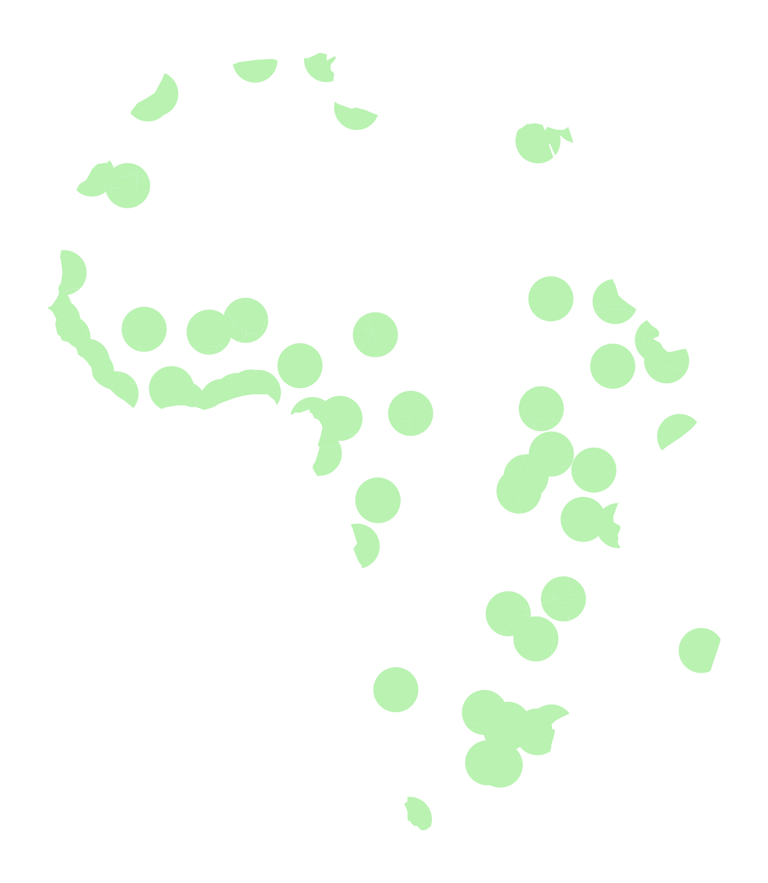

Recap: spatial operations

Spatial join: merge attributes from one data frame to another based on the spatial relationship
Spatial overlay: creating new geometries based on spatial operation between both data frames (and not combining attributes of both data frames)

Example: Exploring trash-related 311 tickets by neighborhood in 2020

Let’s test out our geospatial skills by exploring data for 311 requests in Philadelphia during the pandemic in 2020. We’ll get started by summarizing the data by month and then dive into examining trends by neighborhood.

Find out more…

Trash collection was a big concern in Philadelphia when the pandemic began. Check out this article in the Philadelphia Inquirer for more details!

First, let’s load our data from the data/ folder. I downloaded the data from OpenDataPhilly for tickets from 2020 and trimmed to those requests that have been categorized as “Rubbish/Recyclable Material Collection”. These are tickets related to missed trash pickup by the City’s Streets Department.

# Load the data from a CSV file into a pandas DataFrame
trash_requests_df = pd.read_csv(
    "data/trash_311_requests_2020.csv",  # Use the file path relative to the current folder
)

print("number of requests = ", len(trash_requests_df))

number of requests =  47730

trash_requests_df.head()

	objectid	service_request_id	status	status_notes	service_name	service_code	agency_responsible	service_notice	requested_datetime	updated_datetime	expected_datetime	address	zipcode	media_url	lat	lon
0	8180042	13269656	Closed	NaN	Rubbish/Recyclable Material Collection	SR-ST03	Streets Department	2 Business Days	2020-04-02 19:22:24	2020-04-06 07:02:57	2020-04-06 20:00:00	624 FOULKROD ST	NaN	NaN	40.034389	-75.106518
1	8180043	13266979	Closed	NaN	Rubbish/Recyclable Material Collection	SR-ST03	Streets Department	2 Business Days	2020-04-02 08:40:53	2020-04-06 07:02:58	2020-04-05 20:00:00	1203 ELLSWORTH ST	NaN	NaN	39.936164	-75.163497
2	7744426	13066443	Closed	NaN	Rubbish/Recyclable Material Collection	SR-ST03	Streets Department	2 Business Days	2020-01-02 19:17:55	2020-01-04 05:46:06	2020-01-06 19:00:00	9054 WESLEYAN RD	NaN	NaN	40.058737	-75.018345
3	7744427	13066540	Closed	NaN	Rubbish/Recyclable Material Collection	SR-ST03	Streets Department	2 Business Days	2020-01-03 07:01:46	2020-01-04 05:46:07	2020-01-06 19:00:00	2784 WILLITS RD	NaN	NaN	40.063658	-75.022347
4	7801094	13089345	Closed	NaN	Rubbish/Recyclable Material Collection	SR-ST03	Streets Department	2 Business Days	2020-01-15 13:22:14	2020-01-16 14:03:29	2020-01-16 19:00:00	6137 LOCUST ST	NaN	NaN	39.958186	-75.244732

First, convert to a GeoDataFrame

Remove the requests missing lat/lon coordinates

trash_requests_df = trash_requests_df.dropna(subset=["lat", "lon"])

Create Point objects for each lat and lon combination.

We can use the helper utility function: geopandas.points_from_xy()

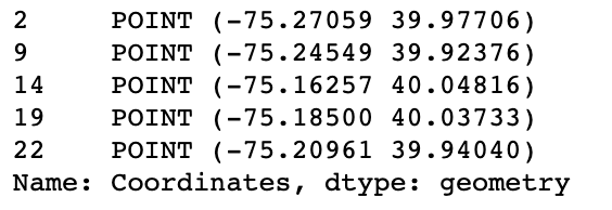
trash_requests_df["geometry"] = gpd.points_from_xy(
    trash_requests_df["lon"], trash_requests_df["lat"]
)

trash_requests_df["geometry"].head()

0    POINT (-75.10652 40.03439)
1    POINT (-75.16350 39.93616)
2    POINT (-75.01835 40.05874)
3    POINT (-75.02235 40.06366)
4    POINT (-75.24473 39.95819)
Name: geometry, dtype: geometry

Now, let’s create our GeoDataFrame object.

Important

Don’t forget to set the CRS manually!
The CRS you specify when creating a GeoDataFrame should tell geopandas what the coordinate system the input data is in.
Usually you will be reading lat/lng coordinates, and will need to specify the crs as EPSG code 4326
You should specify the crs as a string using the syntax: ESPG:4326

Since we’re only using a few EPSG codes in this course, you can usually tell what the CRS is by looking at the values in the Point() objects.

Philadelphia has a latitude of about 40 deg and longitude of about -75 deg.

Our data must be in the usual lat/lng EPSG=4326!

Finally, let’s create our GeoDataFrame:

trash_requests_gdf = gpd.GeoDataFrame(
    trash_requests_df, geometry="geometry", crs="EPSG:4326"
)

Let’s plot the monthly trash requests

Let’s add some new columns based on the “requested_datetime”. Right now, this column is a string, denoted by the dtype “object” in pandas language:

trash_requests_gdf["requested_datetime"].head()

0    2020-04-02 19:22:24
1    2020-04-02 08:40:53
2    2020-01-02 19:17:55
3    2020-01-03 07:01:46
4    2020-01-15 13:22:14
Name: requested_datetime, dtype: object

We can now use the pd.to_datetime() function to convert to a column of special Datetime objects, which have all sorts of useful functionality.

# Convert the requested datetime to a column of Datetime objects
trash_requests_gdf["requested_datetime_dt"] = pd.to_datetime(
    trash_requests_gdf["requested_datetime"]
)

trash_requests_gdf["requested_datetime_dt"].head()

0   2020-04-02 19:22:24
1   2020-04-02 08:40:53
2   2020-01-02 19:17:55
3   2020-01-03 07:01:46
4   2020-01-15 13:22:14
Name: requested_datetime_dt, dtype: datetime64[ns]

It looks like it worked! We have a “datetime64[ns]” dtype for our new column now.

Now that the column is a Datetime Series, it has a special “.dt” attribute. This attribute allows you to quickly extract out parts of the date, e.g., month, day, year, etc., as new columns.

For all of the possible options, see the API docs for pd.Series — take a look at all of the entries that start with pd.Series.dt.

Tip: The strftime() function

For converting datetime objects to strings in a certain format, we can use the “strftime” function (docs). This uses a special syntax to convert the date object to a string with a specific format.

Helpful reference: Use this strftime guide to look up the syntax!

# Use the .dt attribute to extract out the month integer (starting at 0)
trash_requests_gdf["month_int"] = trash_requests_gdf["requested_datetime_dt"].dt.month

# Get the month name too — this is what %B means - (use strftime.org to see the codes!)
trash_requests_gdf["month"] = trash_requests_gdf["requested_datetime_dt"].dt.strftime("%B")

trash_requests_gdf.head()

	objectid	service_request_id	status	status_notes	service_name	service_code	agency_responsible	service_notice	requested_datetime	updated_datetime	expected_datetime	address	zipcode	media_url	lat	lon	geometry	requested_datetime_dt	month_int	month
0	8180042	13269656	Closed	NaN	Rubbish/Recyclable Material Collection	SR-ST03	Streets Department	2 Business Days	2020-04-02 19:22:24	2020-04-06 07:02:57	2020-04-06 20:00:00	624 FOULKROD ST	NaN	NaN	40.034389	-75.106518	POINT (-75.10652 40.03439)	2020-04-02 19:22:24	4	April
1	8180043	13266979	Closed	NaN	Rubbish/Recyclable Material Collection	SR-ST03	Streets Department	2 Business Days	2020-04-02 08:40:53	2020-04-06 07:02:58	2020-04-05 20:00:00	1203 ELLSWORTH ST	NaN	NaN	39.936164	-75.163497	POINT (-75.16350 39.93616)	2020-04-02 08:40:53	4	April
2	7744426	13066443	Closed	NaN	Rubbish/Recyclable Material Collection	SR-ST03	Streets Department	2 Business Days	2020-01-02 19:17:55	2020-01-04 05:46:06	2020-01-06 19:00:00	9054 WESLEYAN RD	NaN	NaN	40.058737	-75.018345	POINT (-75.01835 40.05874)	2020-01-02 19:17:55	1	January
3	7744427	13066540	Closed	NaN	Rubbish/Recyclable Material Collection	SR-ST03	Streets Department	2 Business Days	2020-01-03 07:01:46	2020-01-04 05:46:07	2020-01-06 19:00:00	2784 WILLITS RD	NaN	NaN	40.063658	-75.022347	POINT (-75.02235 40.06366)	2020-01-03 07:01:46	1	January
4	7801094	13089345	Closed	NaN	Rubbish/Recyclable Material Collection	SR-ST03	Streets Department	2 Business Days	2020-01-15 13:22:14	2020-01-16 14:03:29	2020-01-16 19:00:00	6137 LOCUST ST	NaN	NaN	39.958186	-75.244732	POINT (-75.24473 39.95819)	2020-01-15 13:22:14	1	January

Now, let’s group by the month integer and month name, and get the size of the groups using the built-in .size() function of the groupby object:

totals_by_month = trash_requests_gdf.groupby(
    by=["month_int", "month"], as_index=False
).size()

totals_by_month

	month_int	month	size
0	1	January	2710
1	2	February	2067
2	3	March	2460
3	4	April	5778
4	5	May	6572
5	6	June	6485
6	7	July	9627
7	8	August	4466
8	9	September	1704
9	10	October	1335
10	11	November	1729
11	12	December	2757

Note

I’ve used the as_index=False keyword to the groupby() function. This will force the size() function to return a DataFrame instead of having the month column as the index of the resulted groupby operation.

Remember, the columns you group by become the index of the aggregated DataFrame. I often like to have them as columns in the DataFrame instead — the as_index=False flag exists for exactly this problem.

Plot a bar chart with seaborn

For making static bar charts with Python, seaborn’s sns.barplot() is usually the best option!

# Initialize figure/axes
fig, ax = plt.subplots(figsize=(12, 6))

# Plot!
sns.barplot(
    x="month_int",
    y="size",
    data=totals_by_month,
    color="#2176d2",
    ax=ax,
)

ax.set_xticklabels(totals_by_month["month"]);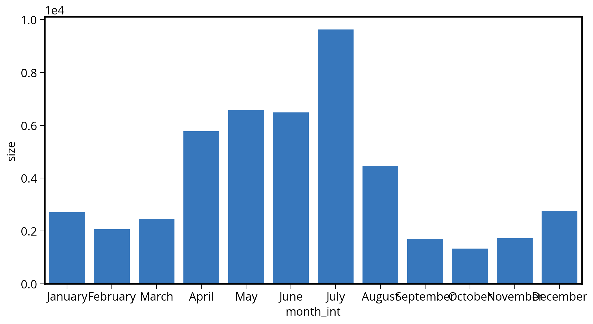

Reference: Let’s improve the aesthetics via matplotlib

The trend is clear in the previous chart, but can we do a better job with the aesthetics? Yes!

For reference, here is a common way to clean up charts in matplotlib:

# Initialize figure/axes
fig, ax = plt.subplots(figsize=(12, 6))

# Plot!
sns.barplot(
    x="month",
    y="size",
    data=totals_by_month,
    color="#2176d2",
    ax=ax,
    order=[
        "January",
        "February",
        "March",
        "April",
        "May",
        "June",
        "July",
        "August",
        "September",
        "October",
        "November",
        "December",
    ],
    zorder=999,  # Make sure the bar charts are on top of the grid
)

# Remove x/y axis labels
ax.set_xlabel("")
ax.set_ylabel("")

# Set the yticks to go from 0 to 10,000 with 2,000 step
ax.set_yticks(np.arange(0, 1e4 + 1, 2e3))

# Format the ytick labels to use a comma and no decimal places
ax.set_yticklabels([f"{yval:,.0f}" for yval in ax.get_yticks()])

# Rotate the xticks
plt.setp(ax.get_xticklabels(), rotation=60)

# Add a grid backgrou d
ax.grid(True, axis="y")

# Remove the top and right axes lines
ax.spines["top"].set_visible(False)
ax.spines["right"].set_visible(False)

# Add a title
ax.set_title(
    "Philadelphia's Trash-Related 311 Requests in 2020", weight="bold", fontsize=16
);

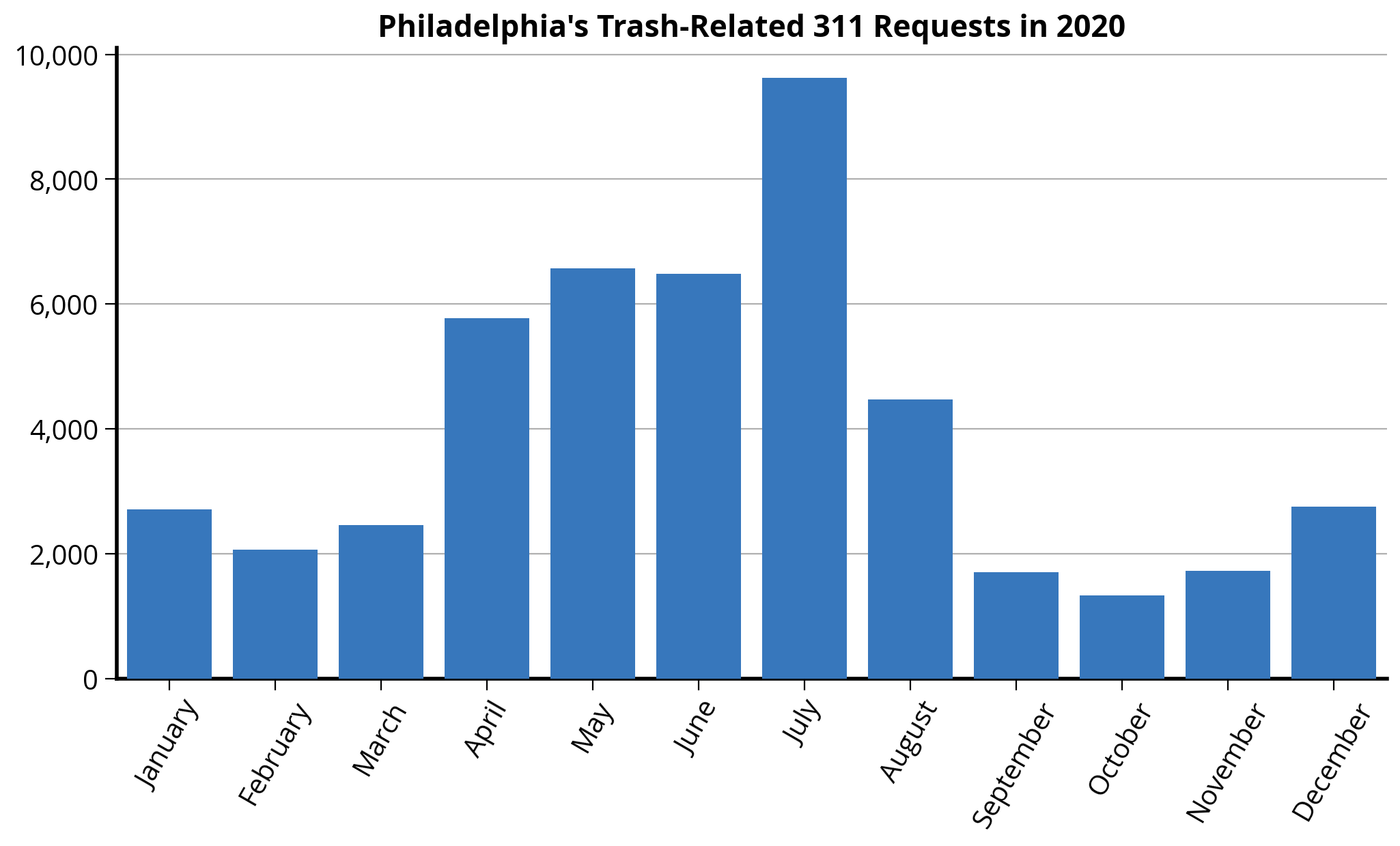
Takeaway: A huge spike in trash related tickets over the summer in 2020!

Tip

This example could come in handy for reference as you work on assignment 2, where you will need to create polished and clear visualizations using both matplotlib and seaborn.

That’s it!

We’ll continue our 311 example next week
More geopandas and geospatial data analysis coming up
See you on Monday next week!

Housekeeping

Agenda for today

Part 1: Vector geospatial data in Python

A couple of terminology notes

Common formats for vector datasets

1. A shapefile

2. The GeoJSON file

Analyzing vector data with GeoPandas

What’s a GeoDataFrame?

We can still leverage the power of pandas…

How does geopandas handle coordinate systems and map projections?

The EPSG=4326 CRS

How to plot all of the geometries at once?

Can we convert to other coordinate systems?

Let’s convert to the Mercator projection

Now let’s plot it!

Which one is your favorite?

Let’s load the city limits for Philadelphia

What’s the CRS?

Saving GeoDataFrames

How about as a CSV file?

Looks similar…

Use shapely to parse the string version of the polygons

Converting from a DataFrame to a GeoDataFrame

Let’s convert back to 4326 and plot

So, when should you use GeoPandas?

When it may not be the best tool:

Part 2: Spatial Relationships and Joins

A quick example

References

1. The spatial join: sjoin()

2. Spatial overlay operation: overlay()

Plot the difference of the two geometries

Plot the intersection of the two geometries

Recap: spatial operations

Example: Exploring trash-related 311 tickets by neighborhood in 2020

First, convert to a GeoDataFrame

Let’s plot the monthly trash requests

Plot a bar chart with seaborn

Reference: Let’s improve the aesthetics via matplotlib

That’s it!

What’s a `GeoDataFrame`?

We can still leverage the power of `pandas`…

How does `geopandas` handle coordinate systems and map projections?

Use `shapely` to parse the string version of the polygons

1. The spatial join: `sjoin()`

2. Spatial overlay operation: `overlay()`