Week 5B
Geospatial Data: Raster

• Section 401
• Wednesday October 4, 2023

# Our usual imports
import altair as alt
import geopandas as gpd
import numpy as np
import pandas as pd
from matplotlib import pyplot as plt

# This will add the .hvplot() function to your DataFrame!
# Import holoviews too
import holoviews as hv
import hvplot.pandas

hv.extension("bokeh")

We’ve already worked with raster data!

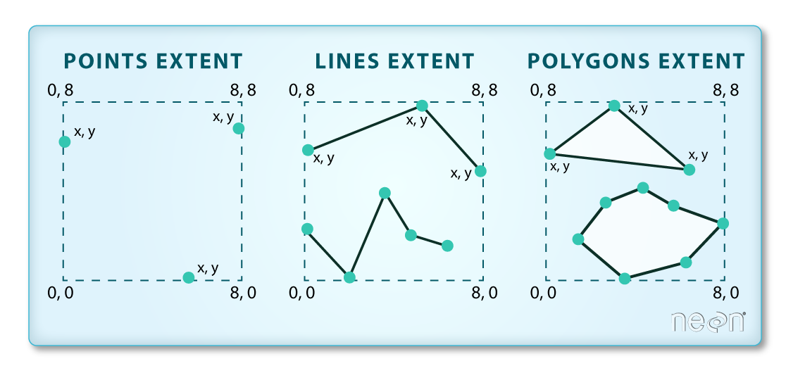
• So far we’ve been working mainly with vector data using geopandas: lines, points, polygons
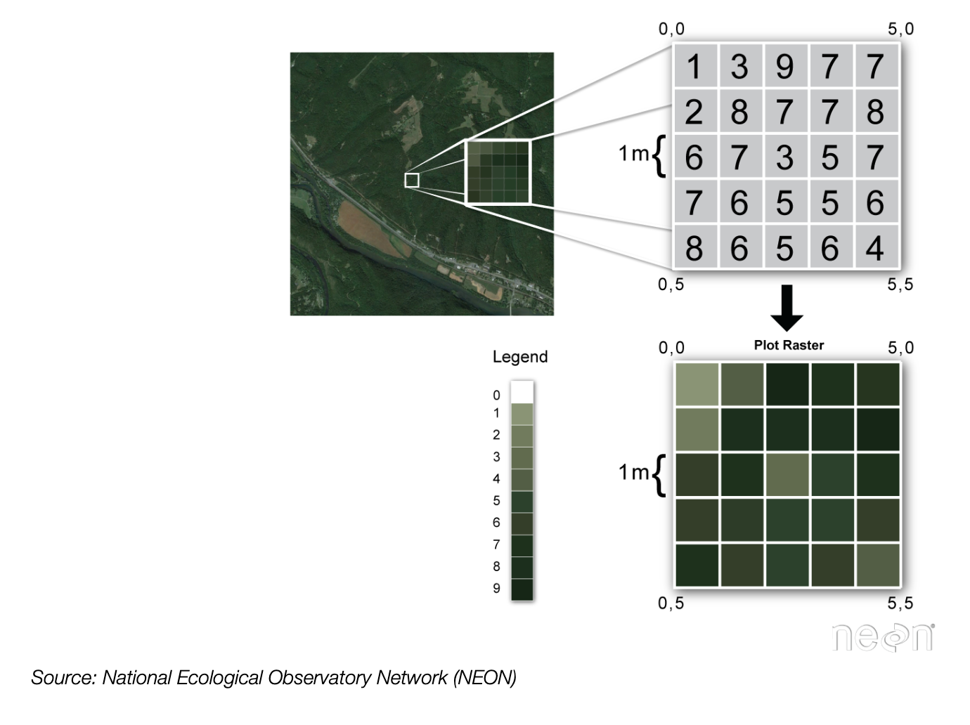
• The basemap tiles we’ve been adding to our hvplot maps are an exampe of raster data
• Raster data:
  • Gridded or pixelated
  • Maps easily to an array — it’s the representation for digital images

Continuous raster examples

• Multispectral satellite imagery, e.g., the Landsat satellite
• Digital Elevation Models (DEMs)
• Maps of canopy height derived from LiDAR data.

Categorical raster examples

• Land cover or land-use maps.
• Tree height maps classified as short, medium, and tall trees.
• Snowcover masks (binary snow or no snow)

Important attributes of raster data

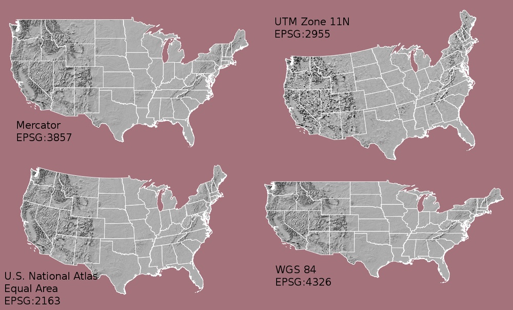
1. The coordinate reference system

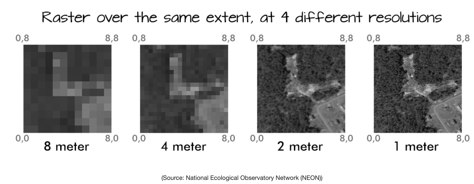
2. Resolution

The spatial distance that a single pixel covers on the ground.

3. Extent

The bounding box that covers the entire extent of the raster data.

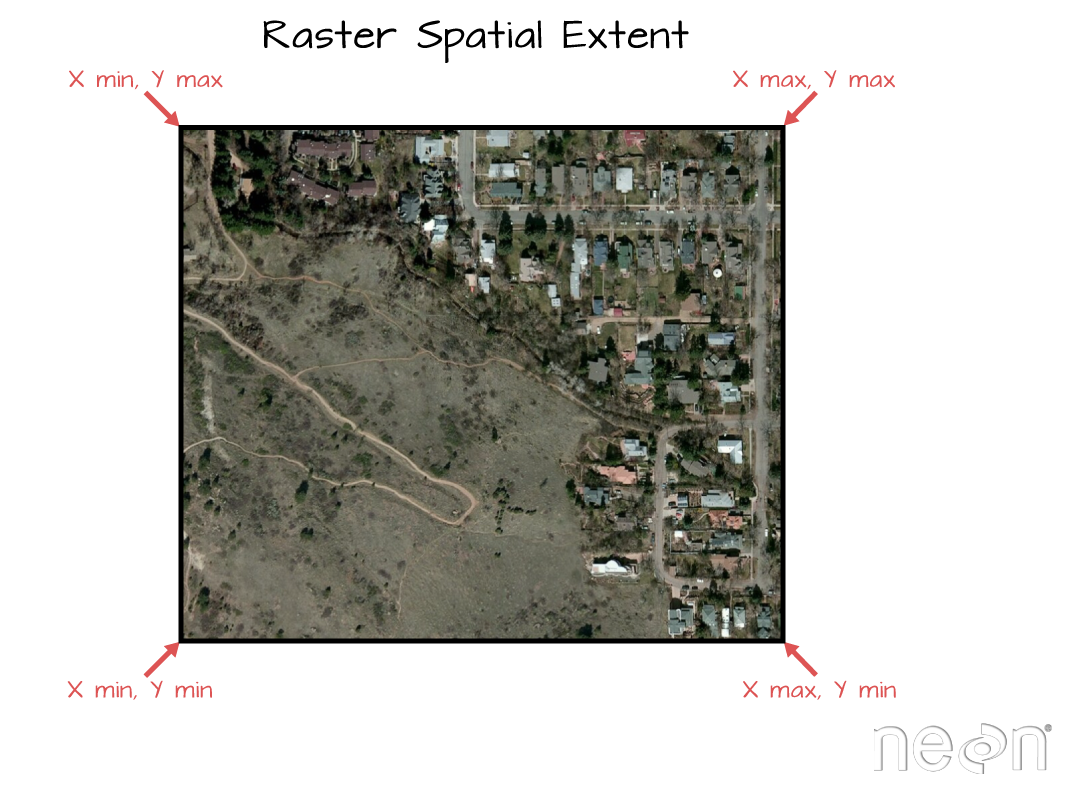
4. Affine transformation

Transform from pixel space to real space

• A mapping from pixel space (rows and columns of the image) to the x and y coordinates defined by the CRS
• Typically a six parameter matrix defining the origin, pixel resolution, and rotation of the raster image

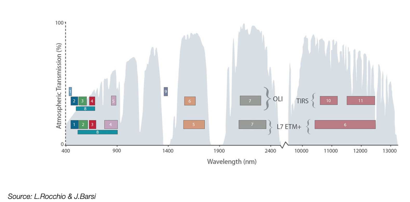
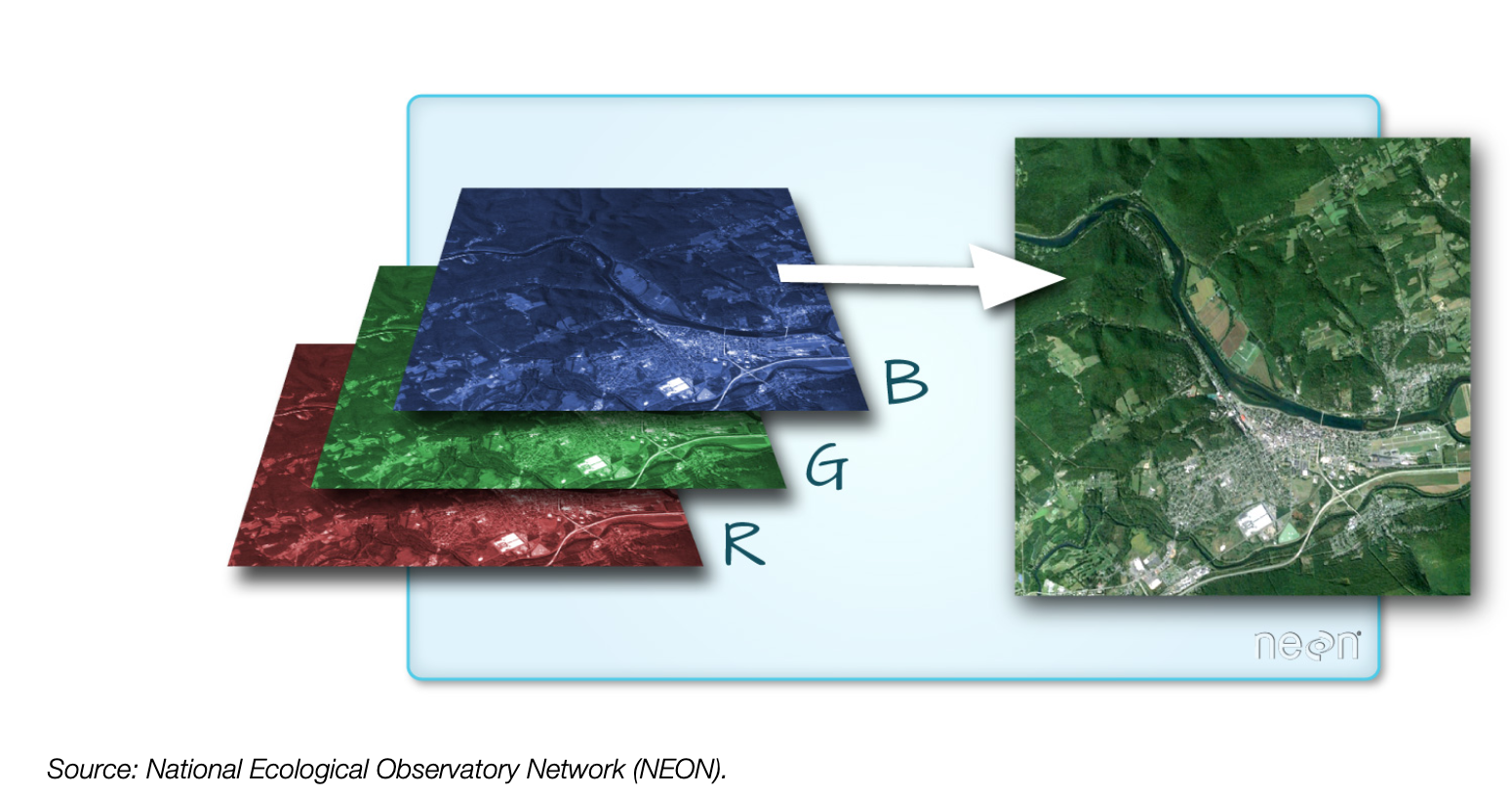
Multi-band raster data

Each band measures the light reflected from different parts of the electromagnetic spectrum.

Color images are multi-band rasters!

The raster format: GeoTIFF

• A standard .tif image format with additional spatial information embedded in the file, which includes metadata for:
  • Geotransform, e.g., extent, resolution
  • Coordinate Reference System (CRS)
  • Values that represent missing data (NoDataValue)

Tools for raster data

• Lots of different options: really just working with arrays
• One of the first options: Geospatial Data Abstraction Library (GDAL)
  • Low level and not really user-friendly
• A more recent, much more Pythonic package: rasterio

We’ll use rasterio for the majority of our raster analysis

Raster data + NumPy

Multi-band raster data is best represented as multi-dimensional arrays. In Python, that means working with NumPy arrays. We’ll work primarily with rasterio today but see a few examples of NumPy arrays.

To learn more about NumPy, we recommend going through the DataCamp course on NumPy. To get free access to DataCamp, see the instructions on the course website.

Part 1: Getting started with rasterio

Analysis is built around the “open()” command which returns a “dataset” or “file handle”

import rasterio as rio

# Open the file and get a file "handle"
landsat = rio.open("./data/landsat8_philly.tif")

landsat

<open DatasetReader name='./data/landsat8_philly.tif' mode='r'>

Let’s check out the metadata

# The CRS
landsat.crs

CRS.from_epsg(32618)

# The bounds
landsat.bounds

BoundingBox(left=476064.3596176505, bottom=4413096.927074196, right=503754.3596176505, top=4443066.927074196)

# The number of bands available
landsat.count

10

# The band numbers that are available
landsat.indexes

(1, 2, 3, 4, 5, 6, 7, 8, 9, 10)

# Number of pixels in the x and y directions
landsat.shape

(999, 923)

# The 6 parameters that map from pixel to real space
landsat.transform

Affine(30.0, 0.0, 476064.3596176505,
       0.0, -30.0, 4443066.927074196)

# All of the meta data
landsat.meta

{'driver': 'GTiff',
 'dtype': 'uint16',
 'nodata': None,
 'width': 923,
 'height': 999,
 'count': 10,
 'crs': CRS.from_epsg(32618),
 'transform': Affine(30.0, 0.0, 476064.3596176505,
        0.0, -30.0, 4443066.927074196)}

Reading data from a file

Tell the file which band to read, starting with 1

# This is a NumPy array!
data = landsat.read(1)

data

array([[10901, 10618, 10751, ..., 12145, 11540, 14954],
       [11602, 10718, 10546, ..., 11872, 11982, 12888],
       [10975, 10384, 10357, ..., 11544, 12318, 12456],
       ...,
       [12281, 12117, 12072, ..., 11412, 11724, 11088],
       [12747, 11866, 11587, ..., 11558, 12028, 10605],
       [11791, 11677, 10656, ..., 10615, 11557, 11137]], dtype=uint16)

Plotting with imshow

We can plot it with matplotlib’s imshow

fig, ax = plt.subplots(figsize=(10, 10))

img = ax.imshow(data)

plt.colorbar(img);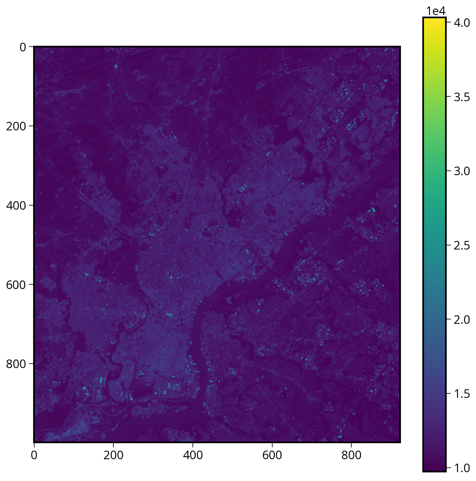

Two improvements

• A log-scale colorbar
• Add the axes extent

1. Adding the axes extent

Note that imshow needs a bounding box of the form: (left, right, bottom, top).

See the documentation for imshow if you forget the right ordering…(I often do!)

2. Using a log-scale color bar

Matplotlib has a built in log normalization…

import matplotlib.colors as mcolors

# Initialize
fig, ax = plt.subplots(figsize=(10, 10))

# Plot the image
img = ax.imshow(
    data,
    # Use a log colorbar scale
    norm=mcolors.LogNorm(),
    # Set the extent of the images
    extent=[
        landsat.bounds.left,
        landsat.bounds.right,
        landsat.bounds.bottom,
        landsat.bounds.top,
    ],
)

# Add a colorbar
plt.colorbar(img);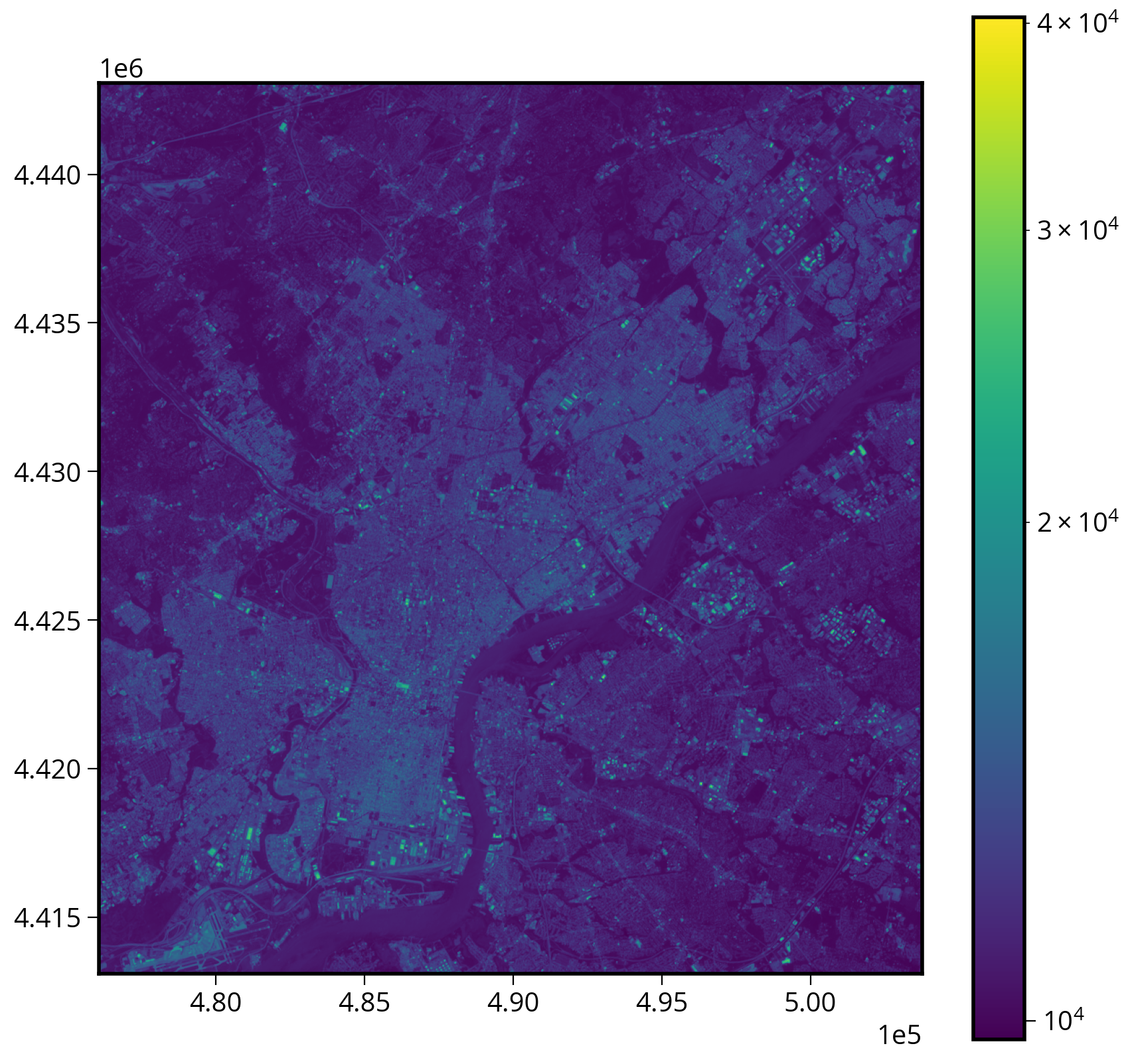

Overlaying vector geometries on raster plots

Two requirements:

1. The CRS of the two datasets must match
2. The extent of the imshow plot must be set properly

Example: Let’s add the city limits

city_limits = gpd.read_file("./data/City_Limits.geojson")

# Convert to the correct CRS!
print(landsat.crs.to_epsg())

32618

city_limits = city_limits.to_crs(epsg=landsat.crs.to_epsg())

# Initialize
fig, ax = plt.subplots(figsize=(10, 10))

# The extent of the data
landsat_extent = [
    landsat.bounds.left,
    landsat.bounds.right,
    landsat.bounds.bottom,
    landsat.bounds.top,
]

# Plot!
img = ax.imshow(data, norm=mcolors.LogNorm(), extent=landsat_extent)

# Add the city limits
city_limits.plot(ax=ax, facecolor="none", edgecolor="white")

# Add a colorbar and turn off axis lines
plt.colorbar(img)
ax.set_axis_off()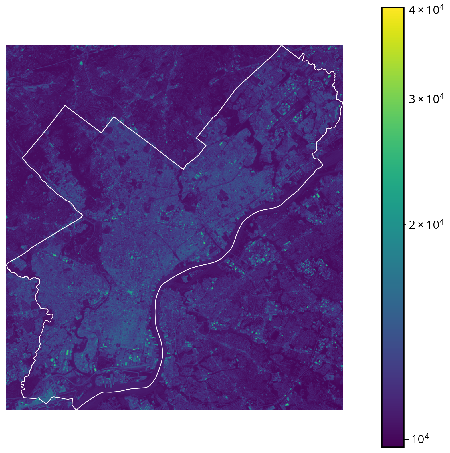

But wait… What band did we plot??

Landsat 8 has 11 bands spanning the electromagnetic spectrum from visible to infrared.

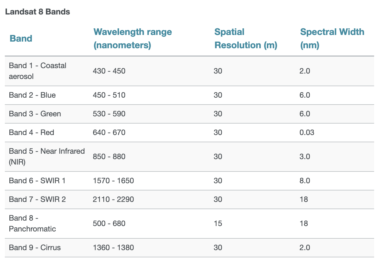
How about a typical RGB color image?

First let’s read the red, blue, and green bands (bands 4, 3, 2):

Note

The .indexes attributes tells us the bands available to be read.

Important: they are NOT zero-indexed!

landsat.indexes

(1, 2, 3, 4, 5, 6, 7, 8, 9, 10)

rgb_data = landsat.read([4, 3, 2])

rgb_data.shape

(3, 999, 923)

Note the data has the shape: (bands, height, width)

rgb_data[0]

array([[ 8908,  7860,  8194, ..., 10387,  9995, 15829],
       [ 9209,  8077,  7657, ...,  9479,  9869, 11862],
       [ 8556,  7534,  7222, ...,  9140, 10283, 10836],
       ...,
       [10514, 10525, 10753, ...,  9760, 10667,  9451],
       [11503, 10408,  9317, ...,  9646, 10929,  8503],
       [10089,  9496,  7862, ...,  8222, 10221, 10160]], dtype=uint16)

fig, axs = plt.subplots(nrows=1, ncols=3, figsize=(12, 6))

cmaps = ["Reds", "Greens", "Blues"]
for i in [0, 1, 2]:
    
    # This subplot axes
    ax = axs[i]

    # Plot
    ax.imshow(rgb_data[i], norm=mcolors.LogNorm(), extent=landsat_extent, cmap=cmaps[i])
    city_limits.plot(ax=ax, facecolor="none", edgecolor="black")

    # Format
    ax.set_axis_off()
    ax.set_title(cmaps[i][:-1])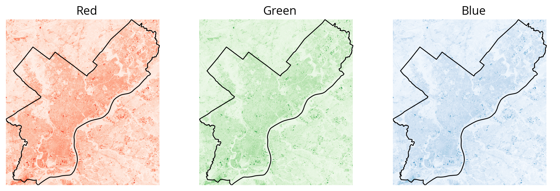

Side note: using subplots in matplotlib

You can specify the subplot layout via the nrows and ncols keywords to plt.subplots. If you have more than one row or column, the function returns: - The figure - The list of axes.

As an example:

fig, axs = plt.subplots(figsize=(10, 3), nrows=1, ncols=3)

Note

When nrows or ncols > 1, I usually name the returned axes variable “axs” vs. the usual case of just “ax”. It’s useful for remembering we got more than one Axes object back!

# This has length 3 for each of the 3 columns!
axs

array([<Axes: >, <Axes: >, <Axes: >], dtype=object)

# Left axes
axs[0]

<Axes: >

# Middle axes
axs[1]

<Axes: >

# Right axes
axs[2]

<Axes: >

Use earthpy to plot the combined color image

A useful utility package to perform the proper re-scaling of pixel values

import earthpy.plot as ep

# Initialize
fig, ax = plt.subplots(figsize=(10, 10))

# Plot the RGB bands
ep.plot_rgb(rgb_data, rgb=(0, 1, 2), ax=ax);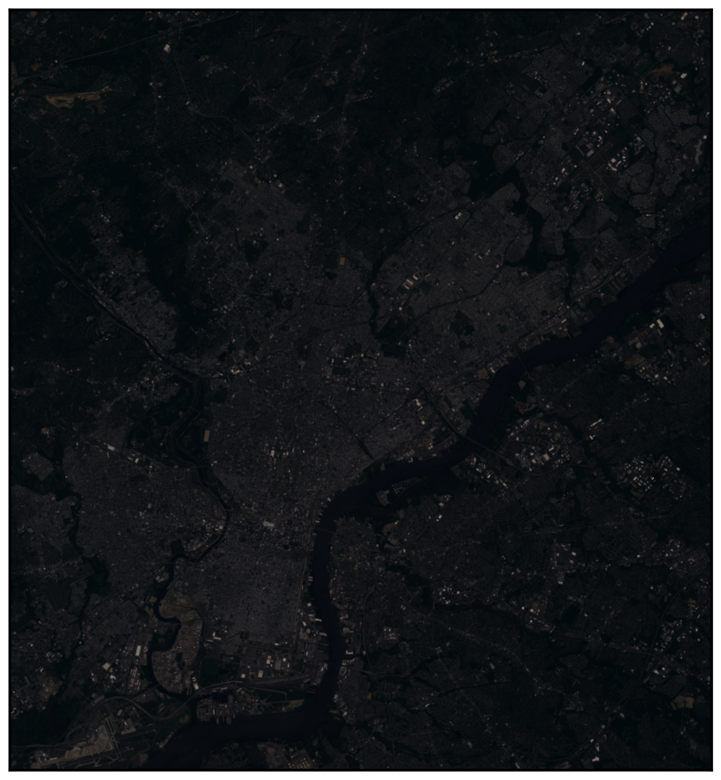

We can “stretch” the data to improve the brightness

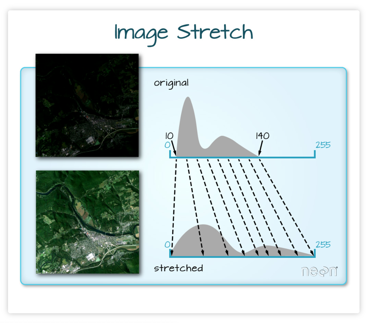
# Initialize
fig, ax = plt.subplots(figsize=(10, 10))

# Plot the RGB bands
ep.plot_rgb(rgb_data, rgb=(0, 1, 2), ax=ax, stretch=True, extent=landsat_extent)

# Add the city limits
city_limits.plot(ax=ax, facecolor="none", edgecolor="crimson", linewidth=4)

# Remove axes
ax.set_axis_off();

Conclusion: Working with multi-band data via rasterio is a bit messy

Can we do better?

Yes!

HoloViz to the rescue…

The xarray package is an alternative way to work with raster data. It’s not as well established as rasterio but has a lot of promising features…

A quick example with xarray

• A fancier version of NumPy arrays
• Designed for gridded data with multiple dimensions
• For raster data, those dimensions are: bands, latitude, longitude, pixel values

import rioxarray  # Adds rasterio engine extension to xarray
import xarray as xr

ds = xr.open_dataset("./data/landsat8_philly.tif", engine="rasterio")

ds

<xarray.Dataset>
Dimensions:      (band: 10, x: 923, y: 999)
Coordinates:
  * band         (band) int64 1 2 3 4 5 6 7 8 9 10
  * x            (x) float64 4.761e+05 4.761e+05 ... 5.037e+05 5.037e+05
  * y            (y) float64 4.443e+06 4.443e+06 ... 4.413e+06 4.413e+06
    spatial_ref  int64 ...
Data variables:
    band_data    (band, y, x) float32 ...

xarray.Dataset

• Dimensions:
  • band: 10
  • x: 923
  • y: 999
• Coordinates: (4)
  • band
    (band)
    int64
    1 2 3 4 5 6 7 8 9 10

    array([ 1,  2,  3,  4,  5,  6,  7,  8,  9, 10])

  • x
    (x)
    float64
    4.761e+05 4.761e+05 ... 5.037e+05

    array([476079.359618, 476109.359618, 476139.359618, ..., 503679.359618,
           503709.359618, 503739.359618])

  • y
    (y)
    float64
    4.443e+06 4.443e+06 ... 4.413e+06

    array([4443051.927074, 4443021.927074, 4442991.927074, ..., 4413171.927074,
           4413141.927074, 4413111.927074])

  • spatial_ref
    ()
    int64
    ...

    crs_wkt :

    PROJCS["WGS 84 / UTM zone 18N",GEOGCS["WGS 84",DATUM["WGS_1984",SPHEROID["WGS 84",6378137,298.257223563,AUTHORITY["EPSG","7030"]],AUTHORITY["EPSG","6326"]],PRIMEM["Greenwich",0,AUTHORITY["EPSG","8901"]],UNIT["degree",0.0174532925199433,AUTHORITY["EPSG","9122"]],AUTHORITY["EPSG","4326"]],PROJECTION["Transverse_Mercator"],PARAMETER["latitude_of_origin",0],PARAMETER["central_meridian",-75],PARAMETER["scale_factor",0.9996],PARAMETER["false_easting",500000],PARAMETER["false_northing",0],UNIT["metre",1,AUTHORITY["EPSG","9001"]],AXIS["Easting",EAST],AXIS["Northing",NORTH],AUTHORITY["EPSG","32618"]]

    semi_major_axis :

    6378137.0

    semi_minor_axis :

    6356752.314245179

    inverse_flattening :

    298.257223563

    reference_ellipsoid_name :

    WGS 84

    longitude_of_prime_meridian :

    0.0

    prime_meridian_name :

    Greenwich

    geographic_crs_name :

    WGS 84

    horizontal_datum_name :

    World Geodetic System 1984

    projected_crs_name :

    WGS 84 / UTM zone 18N

    grid_mapping_name :

    transverse_mercator

    latitude_of_projection_origin :

    0.0

    longitude_of_central_meridian :

    -75.0

    false_easting :

    500000.0

    false_northing :

    0.0

    scale_factor_at_central_meridian :

    0.9996

    spatial_ref :

    PROJCS["WGS 84 / UTM zone 18N",GEOGCS["WGS 84",DATUM["WGS_1984",SPHEROID["WGS 84",6378137,298.257223563,AUTHORITY["EPSG","7030"]],AUTHORITY["EPSG","6326"]],PRIMEM["Greenwich",0,AUTHORITY["EPSG","8901"]],UNIT["degree",0.0174532925199433,AUTHORITY["EPSG","9122"]],AUTHORITY["EPSG","4326"]],PROJECTION["Transverse_Mercator"],PARAMETER["latitude_of_origin",0],PARAMETER["central_meridian",-75],PARAMETER["scale_factor",0.9996],PARAMETER["false_easting",500000],PARAMETER["false_northing",0],UNIT["metre",1,AUTHORITY["EPSG","9001"]],AXIS["Easting",EAST],AXIS["Northing",NORTH],AUTHORITY["EPSG","32618"]]

    GeoTransform :

    476064.3596176505 30.0 0.0 4443066.927074196 0.0 -30.0

    [1 values with dtype=int64]

• Data variables: (1)
  • band_data
    (band, y, x)
    float32
    ...

    AREA_OR_POINT :

    Area

    [9220770 values with dtype=float32]

• Indexes: (3)
  • band
    PandasIndex

    PandasIndex(Int64Index([1, 2, 3, 4, 5, 6, 7, 8, 9, 10], dtype='int64', name='band'))

  • x
    PandasIndex

    PandasIndex(Float64Index([476079.3596176505, 476109.3596176505, 476139.3596176505,
                  476169.3596176505, 476199.3596176505, 476229.3596176505,
                  476259.3596176505, 476289.3596176505, 476319.3596176505,
                  476349.3596176505,
                  ...
                  503469.3596176505, 503499.3596176505, 503529.3596176505,
                  503559.3596176505, 503589.3596176505, 503619.3596176505,
                  503649.3596176505, 503679.3596176505, 503709.3596176505,
                  503739.3596176505],
                 dtype='float64', name='x', length=923))

  • y
    PandasIndex

    PandasIndex(Float64Index([4443051.927074196, 4443021.927074196, 4442991.927074196,
                  4442961.927074196, 4442931.927074196, 4442901.927074196,
                  4442871.927074196, 4442841.927074196, 4442811.927074196,
                  4442781.927074196,
                  ...
                  4413381.927074196, 4413351.927074196, 4413321.927074196,
                  4413291.927074196, 4413261.927074196, 4413231.927074196,
                  4413201.927074196, 4413171.927074196, 4413141.927074196,
                  4413111.927074196],
                 dtype='float64', name='y', length=999))

• Attributes: (0)

type(ds)

xarray.core.dataset.Dataset

Now the magic begins: more hvplot

Still experimental, but very promising — interactive plots with widgets for each band!

import hvplot.xarray

img = ds.hvplot.image(width=700, height=500, cmap="viridis")

img

More magic widgets from hvplot!

That’s it for xarray for now…

More coming in later weeks when we tackle advanced raster examples…

Part 2: Two key raster concepts

• Combining vector + raster data
  • Cropping or masking raster data based on vector polygons
• Raster math and zonal statistics
  • Combining multiple raster data sets
  • Calculating statistics within certain vector polygons

Cropping: let’s trim to just the city limits

Use rasterio’s builtin mask() function:

from rasterio.mask import mask

landsat

<open DatasetReader name='./data/landsat8_philly.tif' mode='r'>

masked, mask_transform = mask(
    dataset=landsat,              # The original raster data
    shapes=city_limits.geometry,  # The vector geometry we want to crop by
    crop=True,                    # Optional: remove pixels not within boundary
    all_touched=True,             # Optional: get all pixels that touch the boudnary
    filled=False,                 # Optional: do not fill cropped pixels with a default value
)

masked

masked_array(
  data=[[[--, --, --, ..., --, --, --],
         [--, --, --, ..., --, --, --],
         [--, --, --, ..., --, --, --],
         ...,
         [--, --, --, ..., --, --, --],
         [--, --, --, ..., --, --, --],
         [--, --, --, ..., --, --, --]],

        [[--, --, --, ..., --, --, --],
         [--, --, --, ..., --, --, --],
         [--, --, --, ..., --, --, --],
         ...,
         [--, --, --, ..., --, --, --],
         [--, --, --, ..., --, --, --],
         [--, --, --, ..., --, --, --]],

        [[--, --, --, ..., --, --, --],
         [--, --, --, ..., --, --, --],
         [--, --, --, ..., --, --, --],
         ...,
         [--, --, --, ..., --, --, --],
         [--, --, --, ..., --, --, --],
         [--, --, --, ..., --, --, --]],

        ...,

        [[--, --, --, ..., --, --, --],
         [--, --, --, ..., --, --, --],
         [--, --, --, ..., --, --, --],
         ...,
         [--, --, --, ..., --, --, --],
         [--, --, --, ..., --, --, --],
         [--, --, --, ..., --, --, --]],

        [[--, --, --, ..., --, --, --],
         [--, --, --, ..., --, --, --],
         [--, --, --, ..., --, --, --],
         ...,
         [--, --, --, ..., --, --, --],
         [--, --, --, ..., --, --, --],
         [--, --, --, ..., --, --, --]],

        [[--, --, --, ..., --, --, --],
         [--, --, --, ..., --, --, --],
         [--, --, --, ..., --, --, --],
         ...,
         [--, --, --, ..., --, --, --],
         [--, --, --, ..., --, --, --],
         [--, --, --, ..., --, --, --]]],
  mask=[[[ True,  True,  True, ...,  True,  True,  True],
         [ True,  True,  True, ...,  True,  True,  True],
         [ True,  True,  True, ...,  True,  True,  True],
         ...,
         [ True,  True,  True, ...,  True,  True,  True],
         [ True,  True,  True, ...,  True,  True,  True],
         [ True,  True,  True, ...,  True,  True,  True]],

        [[ True,  True,  True, ...,  True,  True,  True],
         [ True,  True,  True, ...,  True,  True,  True],
         [ True,  True,  True, ...,  True,  True,  True],
         ...,
         [ True,  True,  True, ...,  True,  True,  True],
         [ True,  True,  True, ...,  True,  True,  True],
         [ True,  True,  True, ...,  True,  True,  True]],

        [[ True,  True,  True, ...,  True,  True,  True],
         [ True,  True,  True, ...,  True,  True,  True],
         [ True,  True,  True, ...,  True,  True,  True],
         ...,
         [ True,  True,  True, ...,  True,  True,  True],
         [ True,  True,  True, ...,  True,  True,  True],
         [ True,  True,  True, ...,  True,  True,  True]],

        ...,

        [[ True,  True,  True, ...,  True,  True,  True],
         [ True,  True,  True, ...,  True,  True,  True],
         [ True,  True,  True, ...,  True,  True,  True],
         ...,
         [ True,  True,  True, ...,  True,  True,  True],
         [ True,  True,  True, ...,  True,  True,  True],
         [ True,  True,  True, ...,  True,  True,  True]],

        [[ True,  True,  True, ...,  True,  True,  True],
         [ True,  True,  True, ...,  True,  True,  True],
         [ True,  True,  True, ...,  True,  True,  True],
         ...,
         [ True,  True,  True, ...,  True,  True,  True],
         [ True,  True,  True, ...,  True,  True,  True],
         [ True,  True,  True, ...,  True,  True,  True]],

        [[ True,  True,  True, ...,  True,  True,  True],
         [ True,  True,  True, ...,  True,  True,  True],
         [ True,  True,  True, ...,  True,  True,  True],
         ...,
         [ True,  True,  True, ...,  True,  True,  True],
         [ True,  True,  True, ...,  True,  True,  True],
         [ True,  True,  True, ...,  True,  True,  True]]],
  fill_value=999999,
  dtype=uint16)

masked.shape

(10, 999, 923)

Let’s plot the masked data:

# Initialize
fig, ax = plt.subplots(figsize=(10, 10))

# Plot the first band
ax.imshow(masked[0], cmap="viridis", extent=landsat_extent)

# Format and add the city limits
city_limits.boundary.plot(ax=ax, color="gray", linewidth=4)
ax.set_axis_off()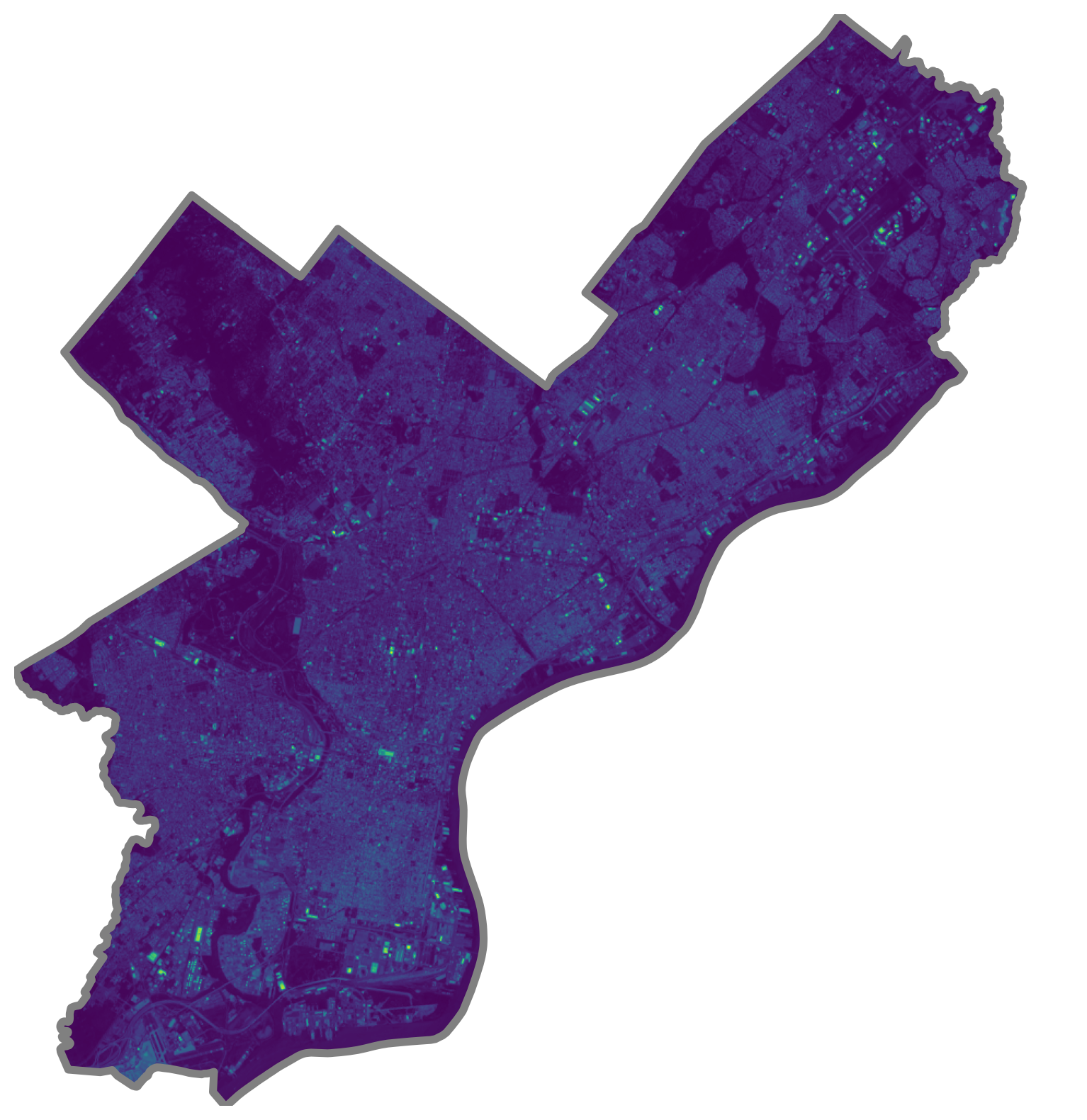

Writing GeoTIFF files

Let’s save our cropped raster data. To save raster data, we need both the array of the data and the proper meta-data.

# The original meta dict
out_meta = landsat.meta

# Call dict.update() to add new key/value pairs
out_meta.update(
    {"height": masked.shape[1], "width": masked.shape[2], "transform": mask_transform}
)

# Print out new meta
print(out_meta)

# Write small image to local Geotiff file
with rio.open("data/cropped_landsat.tif", "w", **out_meta) as dst:
    
    print("dst = ", dst)
    dst.write(masked)
    

{'driver': 'GTiff', 'dtype': 'uint16', 'nodata': None, 'width': 923, 'height': 999, 'count': 10, 'crs': CRS.from_epsg(32618), 'transform': Affine(30.0, 0.0, 476064.3596176505,
       0.0, -30.0, 4443066.927074196)}
dst =  <open DatasetWriter name='data/cropped_landsat.tif' mode='w'>

# Note: dst is now closed — we can't access it any more!
dst

<closed DatasetWriter name='data/cropped_landsat.tif' mode='w'>

Note

We used a context manager above (the “with” statement) to handle the opening and subsequent closing of our new file.

For more info, see this tutorial.

Now, let’s do some raster math

Often called “map algebra”…

The Normalized Difference Vegetation Index

• A normalized index of greenness ranging from -1 to 1, calculated from the red and NIR bands.
• Provides a measure of the amount of live green vegetation in an area

Formula:

NDVI = (NIR - Red) / (NIR + Red)

How to intepret: Healthy vegetation reflects NIR and absorbs visible, so the NDVI for green vegatation is +1

Get the data for the red and NIR bands

NIR is band 5 and red is band 4

masked.shape

(10, 999, 923)

# Note that the indexing here is zero-based, e.g., band 1 is index 0
red = masked[3]
nir = masked[4]

# Where mask = True, pixels are excluded
red.mask

array([[ True,  True,  True, ...,  True,  True,  True],
       [ True,  True,  True, ...,  True,  True,  True],
       [ True,  True,  True, ...,  True,  True,  True],
       ...,
       [ True,  True,  True, ...,  True,  True,  True],
       [ True,  True,  True, ...,  True,  True,  True],
       [ True,  True,  True, ...,  True,  True,  True]])

# Get valid entries
check = np.logical_and(red.mask == False, nir.mask == False)

check
    

array([[False, False, False, ..., False, False, False],
       [False, False, False, ..., False, False, False],
       [False, False, False, ..., False, False, False],
       ...,
       [False, False, False, ..., False, False, False],
       [False, False, False, ..., False, False, False],
       [False, False, False, ..., False, False, False]])

def calculate_NDVI(nir, red):
    """
    Calculate the NDVI from the NIR and red landsat bands
    """

    # Convert to floats
    nir = nir.astype(float)
    red = red.astype(float)

    # Get valid entries
    check = np.logical_and(red.mask == False, nir.mask == False)

    # Where the check is True, return the NDVI, else return NaN
    ndvi = np.where(check, (nir - red) / (nir + red), np.nan)
    
    # Return
    return ndvi

NDVI = calculate_NDVI(nir, red)

fig, ax = plt.subplots(figsize=(10, 10))

# Plot NDVI
img = ax.imshow(NDVI, extent=landsat_extent)

# Format and plot city limits
city_limits.plot(ax=ax, edgecolor="gray", facecolor="none", linewidth=4)
plt.colorbar(img)
ax.set_axis_off()
ax.set_title("NDVI in Philadelphia", fontsize=18);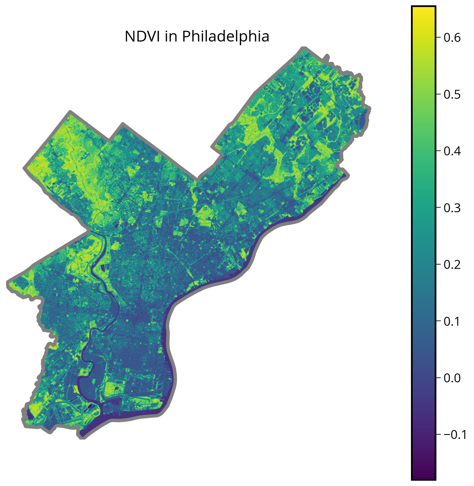

Let’s overlay Philly’s parks

# Read in the parks dataset
parks = gpd.read_file("./data/parks.geojson")

parks.head()

	OBJECTID	ASSET_NAME	SITE_NAME	CHILD_OF	ADDRESS	TYPE	USE_	DESCRIPTION	SQ_FEET	ACREAGE	ZIPCODE	ALLIAS	NOTES	TENANT	LABEL	DPP_ASSET_ID	Shape__Area	Shape__Length	geometry
0	7	Wissahickon Valley Park	Wissahickon Valley Park	Wissahickon Valley Park	NaN	LAND	REGIONAL_CONSERVATION_WATERSHED	NO_PROGRAM	9.078309e+07	2084.101326	19128		MAP	SITE	Wissahickon Valley Park	1357	1.441162e+07	71462.556702	MULTIPOLYGON (((-75.18633 40.02954, -75.18635 ...
1	8	West Fairmount Park	West Fairmount Park	West Fairmount Park		LAND	REGIONAL_CONSERVATION_WATERSHED	NO_PROGRAM	6.078159e+07	1395.358890	19131		MAP	SITE	West Fairmount Park	1714	9.631203e+06	25967.819064	MULTIPOLYGON (((-75.20227 40.00944, -75.20236 ...
2	23	Pennypack Park	Pennypack Park	Pennypack Park		LAND	REGIONAL_CONSERVATION_WATERSHED	NO_PROGRAM	6.023748e+07	1382.867808	19152	Verree Rd Interpretive Center	MAP	SITE	Pennypack Park	1651	9.566914e+06	41487.394790	MULTIPOLYGON (((-75.03362 40.06226, -75.03373 ...
3	24	East Fairmount Park	East Fairmount Park	East Fairmount Park		LAND	REGIONAL_CONSERVATION_WATERSHED	NO_PROGRAM	2.871642e+07	659.240959	19121		MAP	SITE	East Fairmount Park	1713	4.549582e+06	21499.126097	POLYGON ((-75.18103 39.96747, -75.18009 39.967...
4	25	Tacony Creek Park	Tacony Creek Park	Tacony Creek Park		LAND	REGIONAL_CONSERVATION_WATERSHED	NO_PROGRAM	1.388049e+07	318.653500	19120		MAP	SITE	Tacony Creek Park	1961	2.201840e+06	19978.610852	MULTIPOLYGON (((-75.09711 40.01686, -75.09710 ...

Important: make sure you convert to the same CRS as the Landsat data!

# Print out the CRS
parks.crs

<Geographic 2D CRS: EPSG:4326>
Name: WGS 84
Axis Info [ellipsoidal]:
- Lat[north]: Geodetic latitude (degree)
- Lon[east]: Geodetic longitude (degree)
Area of Use:
- name: World.
- bounds: (-180.0, -90.0, 180.0, 90.0)
Datum: World Geodetic System 1984 ensemble
- Ellipsoid: WGS 84
- Prime Meridian: Greenwich

landsat.crs

CRS.from_epsg(32618)

landsat.crs.to_epsg()

32618

# Convert to landsat CRS
parks = parks.to_crs(epsg=landsat.crs.to_epsg())

# Same as: parks = parks.to_crs(epsg=32618)

fig, ax = plt.subplots(figsize=(10, 10))

# Plot NDVI
img = ax.imshow(NDVI, extent=landsat_extent)

# Add the city limits
city_limits.plot(ax=ax, edgecolor="gray", facecolor="none", linewidth=4)

# NEW: add the parks
parks.plot(ax=ax, edgecolor="crimson", facecolor="none", linewidth=2)

# Format and add colorbar
plt.colorbar(img)
ax.set_axis_off()
ax.set_title("NDVI vs. Parks in Philadelphia", fontsize=18);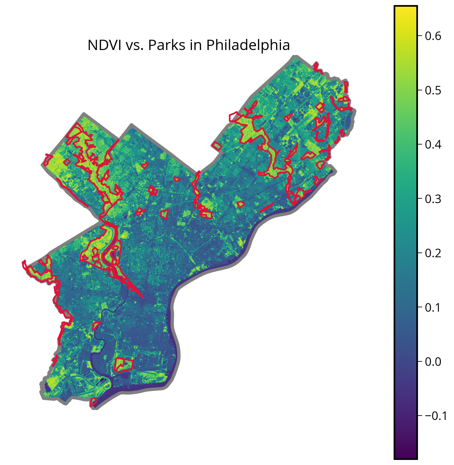

It looks like it worked pretty well!

How about calculating the median NDVI within the park geometries?

This is called zonal statistics. We can use the rasterstats package to do this…

from rasterstats import zonal_stats

stats = zonal_stats(
    parks,  # The vector data
    NDVI,  # The array holding the raster data
    affine=landsat.transform,  # The affine transform for the raster data
    stats=["mean", "median"],  # The stats to compute
    nodata=np.nan,  # Missing data representation
)

The zonal_stats function

Zonal statistics of raster values aggregated to vector geometries.

• First argument: vector data
• Second argument: raster data to aggregated
• Also need to pass the affine transform and the names of the stats to compute

stats

[{'mean': 0.5051087300747117, 'median': 0.521160491292894},
 {'mean': 0.441677258928841, 'median': 0.47791901454593105},
 {'mean': 0.4885958179164529, 'median': 0.5084981442485412},
 {'mean': 0.3756264171005127, 'median': 0.42356277391080177},
 {'mean': 0.45897667566035816, 'median': 0.49204860985900256},
 {'mean': 0.4220467885671325, 'median': 0.46829433706341134},
 {'mean': 0.38363107808041097, 'median': 0.416380868090128},
 {'mean': 0.4330996771737791, 'median': 0.4772304906066629},
 {'mean': 0.45350534061220404, 'median': 0.5015001304461257},
 {'mean': 0.44505112880627273, 'median': 0.4701653486700216},
 {'mean': 0.5017048095513129, 'median': 0.5108644957689836},
 {'mean': 0.23745576631277313, 'median': 0.24259729272419628},
 {'mean': 0.31577818701756977, 'median': 0.3306512446567765},
 {'mean': 0.5300954792288528, 'median': 0.5286783042394015},
 {'mean': 0.4138823685577781, 'median': 0.4604562737642586},
 {'mean': 0.48518030764354636, 'median': 0.5319950233699855},
 {'mean': 0.3154294503884359, 'median': 0.33626983970826585},
 {'mean': 0.4673660755293326, 'median': 0.49301485937514306},
 {'mean': 0.38810332525412405, 'median': 0.4133657898874572},
 {'mean': 0.4408030558751575, 'median': 0.45596817840957254},
 {'mean': 0.5025746121592748, 'median': 0.5077718684805924},
 {'mean': 0.3694178483720184, 'median': 0.3760657145169406},
 {'mean': 0.501111461720193, 'median': 0.5050854708805356},
 {'mean': 0.5262850765386248, 'median': 0.5356888168557536},
 {'mean': 0.48653727784657114, 'median': 0.5100931149323727},
 {'mean': 0.4687375187461541, 'median': 0.49930407348983946},
 {'mean': 0.4708292376095287, 'median': 0.48082651365503404},
 {'mean': 0.4773326667398458, 'median': 0.5156144807640011},
 {'mean': 0.4787564298905878, 'median': 0.49155885289073287},
 {'mean': 0.44870821225970553, 'median': 0.4532736333178444},
 {'mean': 0.28722653079042143, 'median': 0.2989290105395561},
 {'mean': 0.5168607841969154, 'median': 0.5325215878735168},
 {'mean': 0.4725611895576703, 'median': 0.49921839394549977},
 {'mean': 0.46766118115625893, 'median': 0.49758167570710404},
 {'mean': 0.4886459911745514, 'median': 0.5020622294662287},
 {'mean': 0.46017276593316403, 'median': 0.4758438120450033},
 {'mean': 0.4536300550044786, 'median': 0.49233559560028084},
 {'mean': 0.4239182074098442, 'median': 0.4602468966932257},
 {'mean': 0.31202502605597016, 'median': 0.32572928232562837},
 {'mean': 0.2912164528160494, 'median': 0.2946940937582767},
 {'mean': 0.3967233668480246, 'median': 0.3967233668480246},
 {'mean': 0.3226210938878899, 'median': 0.35272291143510365},
 {'mean': 0.4692543355097313, 'median': 0.502843843019927},
 {'mean': 0.2094971073454244, 'median': 0.2736635627619322},
 {'mean': 0.4429390753150177, 'median': 0.49684622604615747},
 {'mean': 0.532656111900622, 'median': 0.5346870838881491},
 {'mean': 0.5053390017291615, 'median': 0.5413888437144251},
 {'mean': 0.500764874094713, 'median': 0.5121577370584547},
 {'mean': 0.4213318206046151, 'median': 0.46379308008197284},
 {'mean': 0.43340892620907207, 'median': 0.4818377611583778},
 {'mean': 0.5069321976848545, 'median': 0.5160336741725328},
 {'mean': 0.4410269675104542, 'median': 0.4870090058426777},
 {'mean': 0.4923323198113241, 'median': 0.5212096391398666},
 {'mean': 0.45403610108483955, 'median': 0.4947035355619755},
 {'mean': 0.2771909854304859, 'median': 0.2843133053564756},
 {'mean': 0.48502792988760635, 'median': 0.5001936488730003},
 {'mean': 0.45418598340923805, 'median': 0.48402058939985293},
 {'mean': 0.32960811687490216, 'median': 0.3285528031290743},
 {'mean': 0.5260210746257522, 'median': 0.5444229172432882},
 {'mean': 0.4445493328049692, 'median': 0.4630808572279276},
 {'mean': 0.4495963972554633, 'median': 0.4858841111806047},
 {'mean': 0.5240412096213553, 'median': 0.5283402835696414},
 {'mean': 0.13767686126646383, 'median': -0.02153756296999343}]

len(stats)

63

len(parks)

63

The returned stats object is a list with one entry for each of the vector polygons (the parks dataset)

Let’s extract out the median value the list of dictionaries:

median_stats = [stats_dict["median"] for stats_dict in stats]

Note: the above cell is equivalent to:

median_stats = []

for stat_dict in stats:
    median_stats.append(stat_dict['median'])

Now, we can add it to the original parks GeoDataFrame as a new column:

# Store the median value in the parks data frame
parks["median_NDVI"] = median_stats

parks.head()

	OBJECTID	ASSET_NAME	SITE_NAME	CHILD_OF	ADDRESS	TYPE	USE_	DESCRIPTION	SQ_FEET	ACREAGE	ZIPCODE	ALLIAS	NOTES	TENANT	LABEL	DPP_ASSET_ID	Shape__Area	Shape__Length	geometry	median_NDVI
0	7	Wissahickon Valley Park	Wissahickon Valley Park	Wissahickon Valley Park	NaN	LAND	REGIONAL_CONSERVATION_WATERSHED	NO_PROGRAM	9.078309e+07	2084.101326	19128		MAP	SITE	Wissahickon Valley Park	1357	1.441162e+07	71462.556702	MULTIPOLYGON (((484101.476 4431051.989, 484099...	0.521160
1	8	West Fairmount Park	West Fairmount Park	West Fairmount Park		LAND	REGIONAL_CONSERVATION_WATERSHED	NO_PROGRAM	6.078159e+07	1395.358890	19131		MAP	SITE	West Fairmount Park	1714	9.631203e+06	25967.819064	MULTIPOLYGON (((482736.681 4428824.579, 482728...	0.477919
2	23	Pennypack Park	Pennypack Park	Pennypack Park		LAND	REGIONAL_CONSERVATION_WATERSHED	NO_PROGRAM	6.023748e+07	1382.867808	19152	Verree Rd Interpretive Center	MAP	SITE	Pennypack Park	1651	9.566914e+06	41487.394790	MULTIPOLYGON (((497133.192 4434667.950, 497123...	0.508498
3	24	East Fairmount Park	East Fairmount Park	East Fairmount Park		LAND	REGIONAL_CONSERVATION_WATERSHED	NO_PROGRAM	2.871642e+07	659.240959	19121		MAP	SITE	East Fairmount Park	1713	4.549582e+06	21499.126097	POLYGON ((484539.743 4424162.545, 484620.184 4...	0.423563
4	25	Tacony Creek Park	Tacony Creek Park	Tacony Creek Park		LAND	REGIONAL_CONSERVATION_WATERSHED	NO_PROGRAM	1.388049e+07	318.653500	19120		MAP	SITE	Tacony Creek Park	1961	2.201840e+06	19978.610852	MULTIPOLYGON (((491712.882 4429633.244, 491713...	0.492049

Make a quick histogram of the median values

They are all positive, indicating an abundance of green vegetation…

# Initialize
fig, ax = plt.subplots(figsize=(8, 6))

# Plot a quick histogram
ax.hist(parks["median_NDVI"], bins="auto")
ax.axvline(x=0, c="k", lw=2)

# Format
ax.set_xlabel("Median NDVI", fontsize=18)
ax.set_ylabel("Number of Parks", fontsize=18);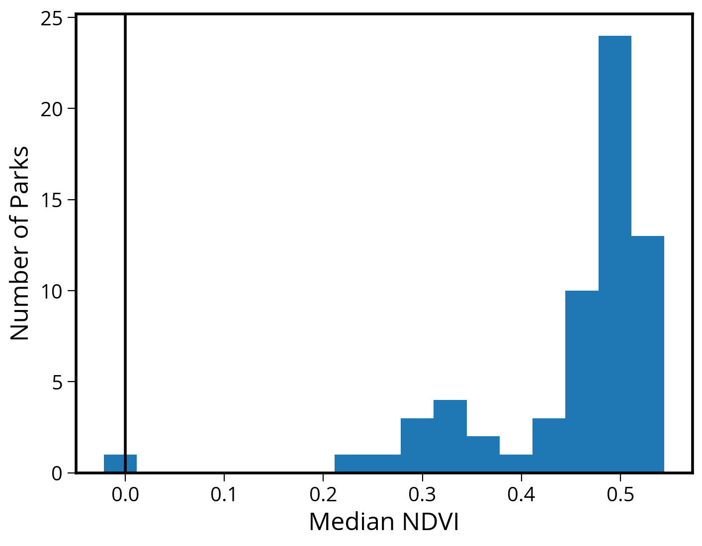

Let’s make a choropleth, too

# Initialize
fig, ax = plt.subplots(figsize=(10, 10))

# Plot the city limits
city_limits.plot(ax=ax, edgecolor="black", facecolor="none", linewidth=4)

# Plot the median NDVI
parks.plot(column="median_NDVI", legend=True, ax=ax, cmap="viridis")

# Format
ax.set_axis_off()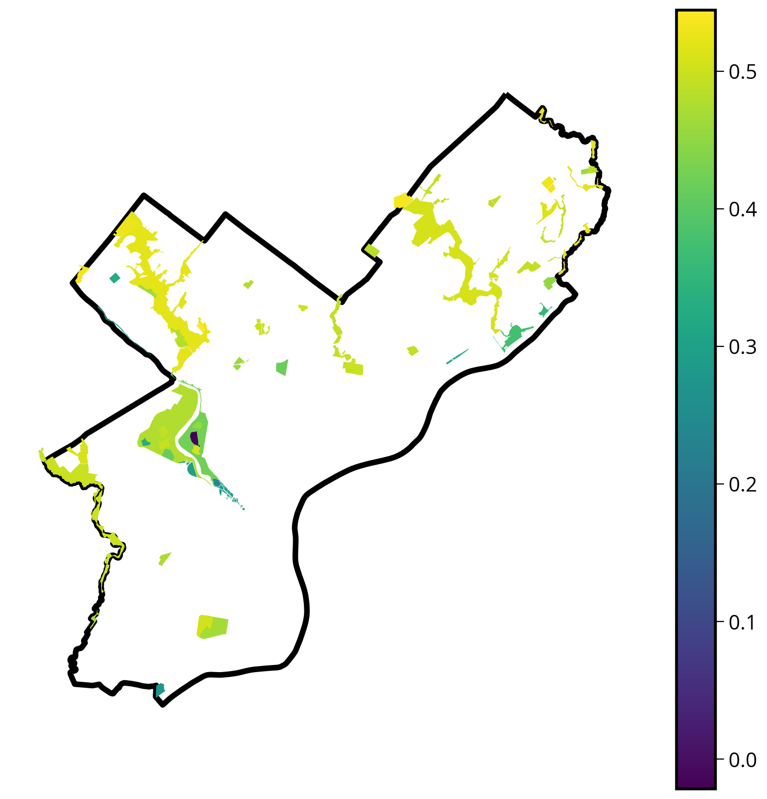

Let’s make it interactive!

Make sure to check the crs!

parks.crs

<Projected CRS: EPSG:32618>
Name: WGS 84 / UTM zone 18N
Axis Info [cartesian]:
- E[east]: Easting (metre)
- N[north]: Northing (metre)
Area of Use:
- name: Between 78°W and 72°W, northern hemisphere between equator and 84°N, onshore and offshore. Bahamas. Canada - Nunavut; Ontario; Quebec. Colombia. Cuba. Ecuador. Greenland. Haiti. Jamaica. Panama. Turks and Caicos Islands. United States (USA). Venezuela.
- bounds: (-78.0, 0.0, -72.0, 84.0)
Coordinate Operation:
- name: UTM zone 18N
- method: Transverse Mercator
Datum: World Geodetic System 1984 ensemble
- Ellipsoid: WGS 84
- Prime Meridian: Greenwich

Note

The CRS is “EPSG:32618” and since it’s not in 4326, we’ll need to specify the “crs=” keyword when plotting!

# trim to only the columns we want to plot
cols = ["median_NDVI", "SITE_NAME", "geometry"]

# Plot the parks colored by median NDVI
p = parks[cols].hvplot.polygons(
    c="median_NDVI", geo=True, crs=32618, cmap="viridis", hover_cols=["SITE_NAME"]
)

# Plot the city limit boundary
cl = city_limits.hvplot.polygons(
    geo=True,
    crs=32618,
    alpha=0,
    line_alpha=1,
    line_color="black",
    hover=False,
    width=700,
    height=600,
)

# combine!
cl * p

Exercise: Measure the median NDVI for each of Philadelphia’s neighborhoods

• Once you measure the median value for each neighborhood, try making the following charts:
  • A histogram of the median values for all neighborhoods
  • Bar graphs with the neighborhoods with the 20 highest and 20 lowest values
  • A choropleth showing the median values across the city

You’re welcome to use matplotlib/geopandas, but encouraged to explore the new hvplot options!

1. Load the neighborhoods data

• A GeoJSON file of Philly’s neighborhoods is available in the “data/” folder

# Load the neighborhoods
hoods = gpd.read_file("./data/zillow_neighborhoods.geojson")

2. Calculate the median NDVI value for each neighborhood

Important

Make sure your neighborhoods GeoDataFrame is in the same CRS as the Landsat data!

# Convert to the landsat CRS
hoods = hoods.to_crs(epsg=landsat.crs.to_epsg())

# Calculate the zonal statistics
stats_by_hood = zonal_stats(
    hoods, # Vector data as GeoDataFrame 
    NDVI, # Raster data as Numpy array
    affine=landsat.transform, # Geospatial info via affine transform
    stats=["mean", "median"]
)

/Users/nhand/mambaforge/envs/musa-550-fall-2023/lib/python3.10/site-packages/rasterstats/io.py:328: NodataWarning: Setting nodata to -999; specify nodata explicitly
  warnings.warn(

stats_by_hood

[{'mean': 0.31392040334687304, 'median': 0.27856594452047934},
 {'mean': 0.18300929138083402, 'median': 0.15571923768967572},
 {'mean': 0.22468445189501648, 'median': 0.17141970412772856},
 {'mean': 0.43065240779519015, 'median': 0.4617488161141866},
 {'mean': 0.318970809622512, 'median': 0.3006904521671514},
 {'mean': 0.25273468406592925, 'median': 0.2483195384843864},
 {'mean': 0.09587147406959982, 'median': 0.08340007053008469},
 {'mean': 0.17925317272000577, 'median': 0.16159209153091308},
 {'mean': 0.16927437879780147, 'median': 0.14856486796785304},
 {'mean': 0.13315183006110315, 'median': 0.0844147036216485},
 {'mean': 0.3032613180748332, 'median': 0.2991018371406554},
 {'mean': 0.3005145367111285, 'median': 0.2983533036011672},
 {'mean': 0.3520402658092766, 'median': 0.36642977306279395},
 {'mean': 0.06850728352663443, 'median': 0.051313743471153465},
 {'mean': 0.1624992167356467, 'median': 0.14594594594594595},
 {'mean': 0.19406263526762074, 'median': 0.19242101469002704},
 {'mean': 0.2495581274514327, 'median': 0.2257300667883086},
 {'mean': 0.04163000301482944, 'median': 0.037030431957658136},
 {'mean': 0.4201038409217668, 'median': 0.4439358649612553},
 {'mean': 0.04225135200774936, 'median': 0.03853493588670528},
 {'mean': 0.2904211760054823, 'median': 0.26470142185928036},
 {'mean': 0.15363805171709244, 'median': 0.12085003697505158},
 {'mean': 0.17152805040632468, 'median': 0.11496098074558328},
 {'mean': 0.42552495036167076, 'median': 0.421658805187364},
 {'mean': 0.3912762229270476, 'median': 0.42212521910111195},
 {'mean': 0.09404645575651284, 'median': 0.07857622565480188},
 {'mean': 0.16491834928991564, 'median': 0.15021318465070516},
 {'mean': 0.3106049986498808, 'median': 0.32583142201834864},
 {'mean': 0.12919644511512735, 'median': 0.11913371378191145},
 {'mean': 0.2915737313903987, 'median': 0.304774440588728},
 {'mean': 0.31787656779796253, 'median': 0.3952783887473803},
 {'mean': 0.195965777548411, 'median': 0.1770113196079921},
 {'mean': 0.05661083180075057, 'median': 0.0499893639651138},
 {'mean': 0.18515284607314653, 'median': 0.17907100357304717},
 {'mean': 0.29283640801624505, 'median': 0.2877666162286677},
 {'mean': 0.1771635174218309, 'median': 0.14970314171568821},
 {'mean': 0.14716619864818462, 'median': 0.11244390749050742},
 {'mean': 0.12469553617180827, 'median': 0.10742619029157832},
 {'mean': 0.18291214109092946, 'median': 0.1216128609630211},
 {'mean': 0.1859549325760223, 'median': 0.17248164686293802},
 {'mean': 0.09016336981602067, 'median': 0.07756515448942505},
 {'mean': 0.14353818825070166, 'median': 0.12901489323524135},
 {'mean': 0.29371646510388005, 'median': 0.2772895703235984},
 {'mean': 0.14261119894987634, 'median': 0.13165141028503385},
 {'mean': 0.160324108968167, 'median': 0.14247544403334816},
 {'mean': 0.19990495725580412, 'median': 0.12561208543149852},
 {'mean': 0.1404895811639291, 'median': 0.11285189208851981},
 {'mean': 0.20007580613997314, 'median': 0.17488414495175872},
 {'mean': 0.29349378771510654, 'median': 0.27647108771333956},
 {'mean': 0.22719447238709786, 'median': 0.21500827689277635},
 {'mean': 0.2620610489891658, 'median': 0.255177304964539},
 {'mean': 0.2540232182541783, 'median': 0.23457093696574202},
 {'mean': 0.3230085712300897, 'median': 0.3263351749539595},
 {'mean': 0.26093326612377477, 'median': 0.2594112652136994},
 {'mean': 0.30115965232695824, 'median': 0.2881442688809087},
 {'mean': 0.10419469673264953, 'median': 0.06574664149015746},
 {'mean': 0.14459843112390638, 'median': 0.1273132150810105},
 {'mean': 0.09983214655943277, 'median': 0.08794976361471002},
 {'mean': 0.14225336243007766, 'median': 0.12302560186487681},
 {'mean': 0.09946071861930077, 'median': 0.07853215389041533},
 {'mean': 0.1452193922659759, 'median': 0.12790372368526273},
 {'mean': 0.11796940950011613, 'median': 0.0776666911598968},
 {'mean': 0.17070274409635827, 'median': 0.15888826411759982},
 {'mean': 0.19068874563285163, 'median': 0.1720531412171591},
 {'mean': 0.09898339526744644, 'median': 0.08963622358746948},
 {'mean': 0.18061992404502175, 'median': 0.15495696640138285},
 {'mean': 0.16533057021385317, 'median': 0.10399253586284649},
 {'mean': 0.11908729513660037, 'median': 0.0588394720437976},
 {'mean': 0.17329359472117273, 'median': 0.10705735100688761},
 {'mean': 0.2337590931600961, 'median': 0.16357100676045763},
 {'mean': 0.21102276332981473, 'median': 0.19582317265976007},
 {'mean': 0.2484378755666938, 'median': 0.23640730014990935},
 {'mean': 0.21642001147674247, 'median': 0.18099201630711736},
 {'mean': 0.129763301389145, 'median': 0.092685120415709},
 {'mean': 0.054999694456918914, 'median': 0.04555942009022349},
 {'mean': 0.18724649877256527, 'median': 0.18596250718311752},
 {'mean': 0.17647253612174493, 'median': 0.14852174323196993},
 {'mean': 0.178385177079417, 'median': 0.16691988950276243},
 {'mean': 0.18817260737171776, 'median': 0.16271241356413235},
 {'mean': 0.13811770403698734, 'median': 0.10897435897435898},
 {'mean': 0.4355159036631469, 'median': 0.44460500963391136},
 {'mean': 0.28184168594689557, 'median': 0.25374251741396553},
 {'mean': 0.22359597758168365, 'median': 0.19391995334256762},
 {'mean': 0.2878755977585209, 'median': 0.25158715762742606},
 {'mean': 0.26728534727462555, 'median': 0.2410734949827748},
 {'mean': 0.28933947460347065, 'median': 0.25559871643303494},
 {'mean': 0.30402279251992353, 'median': 0.30089000839630564},
 {'mean': 0.3922566238548766, 'median': 0.40705882352941175},
 {'mean': 0.10406705198196901, 'median': 0.04374236571919052},
 {'mean': 0.051218927963353054, 'median': 0.04365235141713119},
 {'mean': 0.1723687820405403, 'median': 0.15059755991957824},
 {'mean': 0.33144340218886986, 'median': 0.3072201540212242},
 {'mean': 0.18000603727544026, 'median': 0.1706375749288419},
 {'mean': 0.29408048899874983, 'median': 0.3036726128016789},
 {'mean': 0.08503955870273701, 'median': 0.07407192525923781},
 {'mean': 0.32241253234016937, 'median': 0.31006926588995215},
 {'mean': 0.18205496347967423, 'median': 0.16134765474074647},
 {'mean': 0.12977836123257955, 'median': 0.08590941601457007},
 {'mean': 0.13443566497928924, 'median': 0.11798494025392971},
 {'mean': 0.2033358456620277, 'median': 0.16576007209122687},
 {'mean': 0.32415498788453834, 'median': 0.32617602427921094},
 {'mean': 0.18749910770539593, 'median': 0.17252747252747253},
 {'mean': 0.3193736682602594, 'median': 0.3373959675453564},
 {'mean': 0.3257517503301688, 'median': 0.29360932475884244},
 {'mean': 0.19620976301968188, 'median': 0.1650986741346869},
 {'mean': 0.07896242289726156, 'median': 0.06548635285469223},
 {'mean': 0.09044969459220685, 'median': 0.07117737003058104},
 {'mean': 0.23577910900495405, 'median': 0.2106886253051269},
 {'mean': 0.49002749329456036, 'median': 0.508513798224709},
 {'mean': 0.2967746028243487, 'median': 0.29078296133448145},
 {'mean': 0.23938081232215558, 'median': 0.20916949997582784},
 {'mean': 0.11612617064064894, 'median': 0.10231888964116452},
 {'mean': 0.12195714494535831, 'median': 0.04300298129912368},
 {'mean': 0.20700090460961312, 'median': 0.2064790288239442},
 {'mean': 0.13647293633345284, 'median': 0.12569427247320197},
 {'mean': 0.22309412347829316, 'median': 0.21101490231903636},
 {'mean': 0.10137747100018765, 'median': 0.06563398497986661},
 {'mean': 0.08273584634594518, 'median': 0.06561233591005096},
 {'mean': 0.04312086703340781, 'median': 0.02541695678217338},
 {'mean': 0.2536093586322431, 'median': 0.2311732524352581},
 {'mean': 0.32332895563886144, 'median': 0.32909180590909004},
 {'mean': 0.2277484811069114, 'median': 0.22431761560720143},
 {'mean': 0.1721841184848715, 'median': 0.16058076512244332},
 {'mean': 0.29942596505649405, 'median': 0.29676670038589786},
 {'mean': 0.15940437606074165, 'median': 0.1358949502071032},
 {'mean': 0.12378472816253742, 'median': 0.11830807853171385},
 {'mean': 0.1877499132271723, 'median': 0.17826751036439015},
 {'mean': 0.11943950844267338, 'median': 0.07476532302595251},
 {'mean': 0.17496298489567105, 'median': 0.1659926732955897},
 {'mean': 0.1920977399165265, 'median': 0.16871625674865026},
 {'mean': 0.16337082044518464, 'median': 0.116828342471531},
 {'mean': 0.13862897874493735, 'median': 0.12335431461369693},
 {'mean': 0.17396050138550698, 'median': 0.14759331143448312},
 {'mean': 0.2398879707943406, 'median': 0.2546650763725905},
 {'mean': 0.14397524759541586, 'median': 0.10151342090234151},
 {'mean': 0.11262226656879762, 'median': 0.08519488018434215},
 {'mean': 0.4105827285256272, 'median': 0.43712943197998555},
 {'mean': 0.12208131944943262, 'median': 0.10823104693140795},
 {'mean': 0.10174770697387744, 'median': 0.07673932517169305},
 {'mean': 0.13941350910672, 'median': 0.11942396096727109},
 {'mean': 0.20263947878478583, 'median': 0.1750341162105868},
 {'mean': 0.42006022571388996, 'median': 0.4711730560719998},
 {'mean': 0.19283089059664163, 'median': 0.12246812581863598},
 {'mean': 0.06900296739992386, 'median': 0.0563680745433852},
 {'mean': 0.16839264609586674, 'median': 0.1653832567997174},
 {'mean': 0.20260798649692677, 'median': 0.17538042425378467},
 {'mean': 0.4514355509481655, 'median': 0.4945924206514285},
 {'mean': 0.08120602841441002, 'median': 0.05459630483539914},
 {'mean': 0.3175258476394397, 'median': 0.3184809770175624},
 {'mean': 0.23161067366700408, 'median': 0.22945830797321973},
 {'mean': 0.32557766938441296, 'median': 0.3120613068393747},
 {'mean': 0.5017692669135977, 'median': 0.5207786535525264},
 {'mean': 0.17652187824323134, 'median': 0.14554151586614233},
 {'mean': 0.32586693646536, 'median': 0.3296868690576704},
 {'mean': 0.2076776587799097, 'median': 0.20473126032547465},
 {'mean': 0.2604215070389401, 'median': 0.24160812708080265},
 {'mean': 0.263077089015587, 'median': 0.25120875995449377},
 {'mean': 0.16880134097818922, 'median': 0.15243747069084695}]

# Store the median value in the neighborhood data frame
hoods["median_NDVI"] = [stats_dict["median"] for stats_dict in stats_by_hood]

hoods.head()

	ZillowName	geometry	median_NDVI
0	Academy Gardens	POLYGON ((500127.271 4434899.076, 500464.133 4...	0.278566
1	Airport	POLYGON ((483133.506 4415847.150, 483228.716 4...	0.155719
2	Allegheny West	POLYGON ((485837.663 4428133.600, 485834.655 4...	0.171420
3	Andorra	POLYGON ((480844.652 4435202.290, 480737.832 4...	0.461749
4	Aston Woodbridge	POLYGON ((499266.779 4433715.944, 499265.975 4...	0.300690

3. Make a histogram of median values

# Initialize
fig, ax = plt.subplots(figsize=(8, 6))

# Plot a quick histogram
ax.hist(hoods["median_NDVI"], bins="auto")
ax.axvline(x=0, c="k", lw=2)

# Format
ax.set_xlabel("Median NDVI", fontsize=18)
ax.set_ylabel("Number of Neighborhoods", fontsize=18);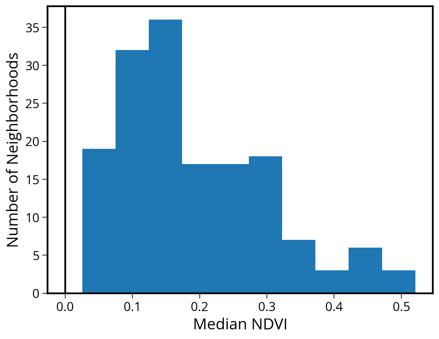

4. Plot a (static) choropleth map

# Initialize
fig, ax = plt.subplots(figsize=(10, 10))

# Plot the city limits
city_limits.plot(ax=ax, edgecolor="black", facecolor="none", linewidth=4)

# Plot the median NDVI
hoods.plot(column="median_NDVI", legend=True, ax=ax)

# Format
ax.set_axis_off()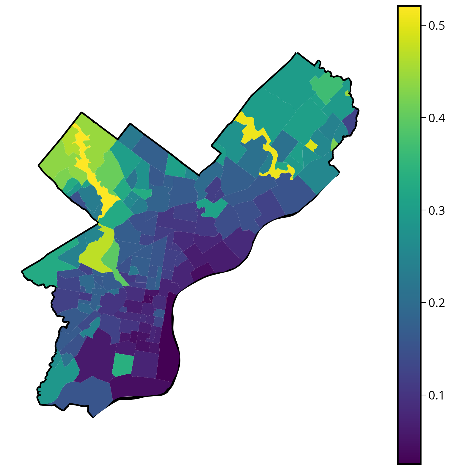

5. Plot an (interactive) choropleth map

You can use your favorite library: hvplot, altair, or geopandas. Solutions will include examples of all three!

With hvplot

# trim to only the columns we want to plot
cols = ["median_NDVI", "ZillowName", "geometry"]

# Plot 
hoods[cols].hvplot.polygons(
    c="median_NDVI",
    geo=True,
    crs=32618,
    frame_width=600,
    frame_height=600,
    cmap="viridis",
    hover_cols=["ZillowName"],
)

With geopandas

# Plot the parks colored by median NDVI
hoods.explore(column="median_NDVI", cmap="viridis", tiles="Cartodb positron")

Make this Notebook Trusted to load map: File -> Trust Notebook

With altair

# trim to only the columns we want to plot
cols = ["median_NDVI", "ZillowName", "geometry"]

(
    alt.Chart(hoods[cols].to_crs(epsg=3857))
    .mark_geoshape()
    .encode(
        color=alt.Color(
            "median_NDVI",
            scale=alt.Scale(scheme="viridis"),
            legend=alt.Legend(title="Median NDVI"),
        ),
        tooltip=["ZillowName", "median_NDVI"],
    )
    .project(type="identity", reflectY=True)
)

6. Challenges

A few extra analysis pieces as an extra challenge. Let’s explore the neighborhoods with the highest and lowest median NDVI values.

6A. Plot a bar chart of the neighborhoods with the top 20 largest median values

With hvplot:

# calculate the top 20
cols = ["ZillowName", "median_NDVI"]
top20 = hoods[cols].sort_values("median_NDVI", ascending=False).head(n=20)

top20.hvplot.bar(x="ZillowName", y="median_NDVI", rot=90, height=400)

With altair:

(
    alt.Chart(top20)
    .mark_bar()
    .encode(
        x=alt.X("ZillowName", sort="-y"),  # Sort in descending order by y
        y="median_NDVI",
        tooltip=["ZillowName", "median_NDVI"],
    )
    .properties(width=800)
)

6B. Plot a bar chart of the neighborhoods with the bottom 20 largest median values

With hvplot:

cols = ["ZillowName", "median_NDVI"]
bottom20 = hoods[cols].sort_values("median_NDVI", ascending=True).tail(n=20)


bottom20.hvplot.bar(x="ZillowName", y="median_NDVI", rot=90, height=300, width=600)

With altair:

(
    alt.Chart(bottom20)
    .mark_bar()
    .encode(
        x=alt.X("ZillowName", sort="y"),  # Sort in ascending order by y
        y="median_NDVI",
        tooltip=["ZillowName", "median_NDVI"],
    )
    .properties(width=800)
)

That’s it!

• Coming up next: moving on to our “getting data” modules with APIs and web scraping
• See you on Monday!