Week 7A
Getting Data, Part 2: Working with APIs

Section 401
Monday Oct 16, 2023

Week #7 Agenda

Introduction to APIs
Natural language processing via Philly’s 311 API
- Word frequencies
- Sentiment analysis
Pulling census data and shape files using Python

Important

Update your local environment!

Small update to the course’s Python environment
Update the environment on your laptop using these instructions on course website

import geopandas as gpd
import holoviews as hv
import hvplot.pandas
import numpy as np
import pandas as pd
import seaborn as sns
from matplotlib import pyplot as plt

# Show all columns
pd.options.display.max_columns = 999

Part 1: Introduction to APIs

Or, how to pull data from the web using Python

Application programming interface (API):

(noun): A particular set of rules and specifications that software programs can follow to communicate with each other and exchange data.

Example APIs

Socrata Open Data: https://dev.socrata.com/
Open Data Philly: https://opendataphilly.org
US Census Bureau: https://www.census.gov/data/developers/data-sets.html
Bureau of Labor Statistics: https://www.bls.gov/developers/
US Geological Survey: https://www.usgs.gov/products/data-and-tools/apis
US Environmental Protection Agency: https://www.epa.gov/enviro/web-services
Google APIs: https://console.cloud.google.com/apis/library
Facebook: https://developers.facebook.com/docs/apis-and-sdks/
Twitter: https://developer.twitter.com/en/docs/api-reference-index.html (RIP 💀)
Foursquare: https://developer.foursquare.com/
Instagram: https://www.instagram.com/developer/
Yelp: https://www.yelp.com/developers

Note

When accessing data via API, many services will require you to register an API key to prevent you from overloading the service with requests.

Example #1: Automated data feeds

The simplest form of API is when data providers maintain data files via a URL that are automatically updated with new data over time.

USGS real-time earthquake feeds

This is an API for near-real-time data about earthquakes, and data is provided in GeoJSON format over the web.

The API has a separate endpoint for each version of the data that users might want. No authentication is required.

API documentation:

http://earthquake.usgs.gov/earthquakes/feed/v1.0/geojson.php

Sample API endpoint, for magnitude 4.5+ earthquakes in past day:

http://earthquake.usgs.gov/earthquakes/feed/v1.0/summary/4.5_day.geojson

GeoPandas can read GeoJSON files from the web directly. Simply pass the URL to the gpd.read_file() function:

# Download data on magnitude 2.5+ quakes from the past week
endpoint_url = (
    "http://earthquake.usgs.gov/earthquakes/feed/v1.0/summary/2.5_week.geojson"
)
earthquakes = gpd.read_file(endpoint_url)

earthquakes.head()

	id	mag	place	time	updated	tz	url	detail	felt	cdi	mmi	alert	status	sig	net	code	ids	sources	types	nst	dmin	rms	gap	magType	type	title	geometry
0	us6000lg18	4.50	Mariana Islands region	1697495094131	1697496425040	NaN	https://earthquake.usgs.gov/earthquakes/eventp...	https://earthquake.usgs.gov/earthquakes/feed/v...	NaN	NaN	NaN	NaN	reviewed	312	us	6000lg18	,us6000lg18,	,us,	,origin,phase-data,	27.0	3.168	0.46	165.0	mb	earthquake	M 4.5 - Mariana Islands region	POINT Z (147.53230 17.94240 10.00000)
1	ak023daay0wr	2.50	Kodiak Island region, Alaska	1697491317711	1697493637040	NaN	https://earthquake.usgs.gov/earthquakes/eventp...	https://earthquake.usgs.gov/earthquakes/feed/v...	NaN	NaN	NaN	NaN	automatic	96	ak	023daay0wr	,us6000lg02,ak023daay0wr,	,us,ak,	,origin,phase-data,	NaN	NaN	1.16	NaN	ml	earthquake	M 2.5 - Kodiak Island region, Alaska	POINT Z (-153.12000 57.13730 0.00000)
2	ak023daavntz	2.50	99 km SE of Old Harbor, Alaska	1697490628779	1697493347040	NaN	https://earthquake.usgs.gov/earthquakes/eventp...	https://earthquake.usgs.gov/earthquakes/feed/v...	NaN	NaN	NaN	NaN	reviewed	96	ak	023daavntz	,us6000lg05,ak023daavntz,	,us,ak,	,origin,phase-data,	NaN	NaN	1.54	NaN	ml	earthquake	M 2.5 - 99 km SE of Old Harbor, Alaska	POINT Z (-152.13590 56.57760 15.00000)
3	hv73610612	2.86	21 km W of Volcano, Hawaii	1697485792740	1697487909640	NaN	https://earthquake.usgs.gov/earthquakes/eventp...	https://earthquake.usgs.gov/earthquakes/feed/v...	NaN	NaN	NaN	NaN	reviewed	126	hv	73610612	,us6000lfz9,hv73610612,	,us,hv,	,origin,phase-data,	53.0	NaN	0.12	68.0	ml	earthquake	M 2.9 - 21 km W of Volcano, Hawaii	POINT Z (-155.44050 19.46667 6.83000)
4	us6000lfyi	4.30	La Rioja-San Juan border region, Argentina	1697482144060	1697483277040	NaN	https://earthquake.usgs.gov/earthquakes/eventp...	https://earthquake.usgs.gov/earthquakes/feed/v...	NaN	NaN	NaN	NaN	reviewed	284	us	6000lfyi	,us6000lfyi,	,us,	,moment-tensor,origin,phase-data,	48.0	1.728	1.08	81.0	mwr	earthquake	M 4.3 - La Rioja-San Juan border region, Argen...	POINT Z (-68.25610 -29.32270 39.71600)

Let’s explore the data interactively with Folium:

earthquakes.explore()

Make this Notebook Trusted to load map: File -> Trust Notebook

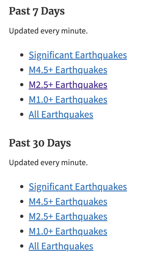
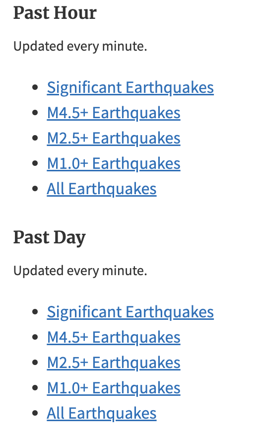
Lots of other automated feeds available, updated every minute:

Example #2: The CARTO API

Philadelphia hosts the majority of its open data on OpenDataPhilly in the cloud using CARTO
They provide an API to download the data
You can access the API documentation on the dataset page on OpenDataPhilly

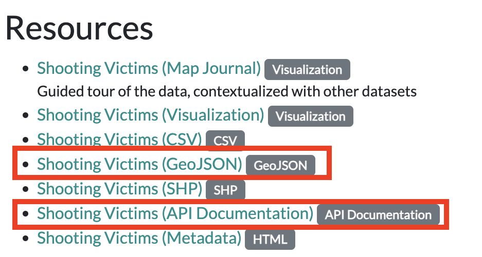
For example: shooting victims in Philadelphia

https://www.opendataphilly.org/dataset/shooting-victims

and the API documentation:

https://cityofphiladelphia.github.io/carto-api-explorer/#shootings

Let’s take a look at the download URL for the data in the GeoJSON format:

The anatomy of an API request

Base URL: shown in blue
?: shown in purple; it separates the base URL from the query parameters
Query parameters: underlined in red; these parameters allow the user to customize the data response
&: underlined in green; the separator between the query parameters

So, let’s break down the URL into its component parts:

# The API endpoint
carto_api_endpoint = "https://phl.carto.com/api/v2/sql"

# The query parameters
params = {
    "q": "SELECT * FROM shootings",
    "format": "geojson",
    "skipfields": "cartodb_id",
    # Note: we won't need the filename parameter, since we're not saving the data to a file
    # "filename": "shootings"
}

Note: SQL Queries

The q parameter is a SQL query. It allows you to select a specific subset of data from the larger database.

CARTO API documentation: https://carto.com/developers/sql-api/

SQL documentation: https://www.postgresql.org/docs/9.1/sql.html

General Query Syntax

SELECT [field names] FROM [table name] WHERE [query]

Let’s try it out in Python

We’ll use Python’s requests library to use a “get” request to query the API endpoint with our desired query. Similar to our web scraping requests!

import requests

Let’s make the get request and pass the query parameters via the params keyword:

response = requests.get(carto_api_endpoint, params=params)

response

<Response [200]>

# Get the returned data in JSON format
# This is a dictionary
features = response.json()

type(features)

dict

# What are the keys?
list(features.keys())

['type', 'features']

features["type"]

'FeatureCollection'

# Let's look at the first feature
features["features"][0]

{'type': 'Feature',
 'geometry': {'type': 'Point', 'coordinates': [-75.162274, 39.988715]},
 'properties': {'objectid': 10797984,
  'year': 2020,
  'dc_key': '202022062735.0',
  'code': '411',
  'date_': '2020-09-12T00:00:00Z',
  'time': '21:04:00',
  'race': 'W',
  'sex': 'M',
  'age': '53',
  'wound': 'Foot',
  'officer_involved': 'N',
  'offender_injured': 'N',
  'offender_deceased': 'N',
  'location': '18TH & DAUPHIN ST',
  'latino': 1,
  'point_x': -75.16227376,
  'point_y': 39.98871456,
  'dist': '22',
  'inside': 0,
  'outside': 1,
  'fatal': 0}}

Use the GeoDataFrame.from_features() function to create a GeoDataFrame.

shootings = gpd.GeoDataFrame.from_features(features, crs="EPSG:4326")

Important

Don’t forget to specify the CRS of the input data when using GeoDataFrame.from_features().

shootings.head()

	geometry	objectid	year	dc_key	code	date_	time	race	sex	age	wound	officer_involved	offender_injured	offender_deceased	location	latino	point_x	point_y	dist	outside	fatal
0	POINT (-75.16227 39.98871)	10797984	2020	202022062735.0	411	2020-09-12T00:00:00Z	21:04:00	W	M	53	Foot	N	N	N	18TH & DAUPHIN ST	1.0	-75.162274	39.988715	22	1.0	0.0
1	POINT (-75.14885 39.98795)	10797985	2020	202022062782.0	111	2020-09-13T00:00:00Z	10:50:00	W	M	22	Multiple/Head	N	N	N	1000 BLOCK W ARIZONA ST	0.0	-75.148851	39.987952	22	1.0	1.0
2	POINT (-75.16062 39.98691)	10797986	2020	202022063114.0	411	2020-09-14T00:00:00Z	20:46:00	B	M	42	Multiple	N	N	N	1600 BLOCK SUSQUEHANNA AVE	0.0	-75.160616	39.986907	22	1.0	0.0
3	POINT (-75.16062 39.98691)	10797987	2020	202022063126.0	411	2020-09-14T00:00:00Z	20:46:00	B	M	17	Buttocks	N	N	N	1600 BLOCK SUSQUEHANNA AVE	0.0	-75.160616	39.986907	22	1.0	0.0
4	POINT (-75.15398 39.98373)	10797988	2020	202022063470.0	111	2020-09-16T00:00:00Z	12:10:00	B	M	39	Head	N	N	N	2000 BLOCK W SUSQUEHANNA AVE	0.0	-75.153980	39.983726	22	1.0	1.0

At-Home Exercise: Visualizing shootings data

Step 1: Prep the data

Drop rows where the geometry is NaN
Convert to a better CRS (e.g., 3857)
Load city limits from Open Data Philly and trim to those only within city limits (some shootings have wrong coordinates, outside Philadelphia!)

# make sure we remove missing geometries
shootings = shootings.dropna(subset=["geometry"])

# convert to a better CRS
shootings = shootings.to_crs(epsg=3857)

city_limits = gpd.read_file(
    "https://opendata.arcgis.com/datasets/405ec3da942d4e20869d4e1449a2be48_0.geojson"
).to_crs(epsg=3857)

# Remove any shootings that are outside the city limits
shootings = gpd.sjoin(shootings, city_limits, predicate="within", how="inner").drop(
    columns=["index_right"]
)

Step 2: Plot the points

A quick plot with geopandas to show the shootings as points, and overlay Philadelphia ZIP codes.

# From Open Data Philly
zip_codes = gpd.read_file(
    "https://opendata.arcgis.com/datasets/b54ec5210cee41c3a884c9086f7af1be_0.geojson"
).to_crs(epsg=3857)

fig, ax = plt.subplots(figsize=(6, 6))

# ZIP Codes
zip_codes.to_crs(epsg=3857).plot(ax=ax, facecolor="none", edgecolor="black")

# Shootings
shootings.plot(ax=ax, color="crimson", markersize=10, alpha=0.4)
ax.set_axis_off()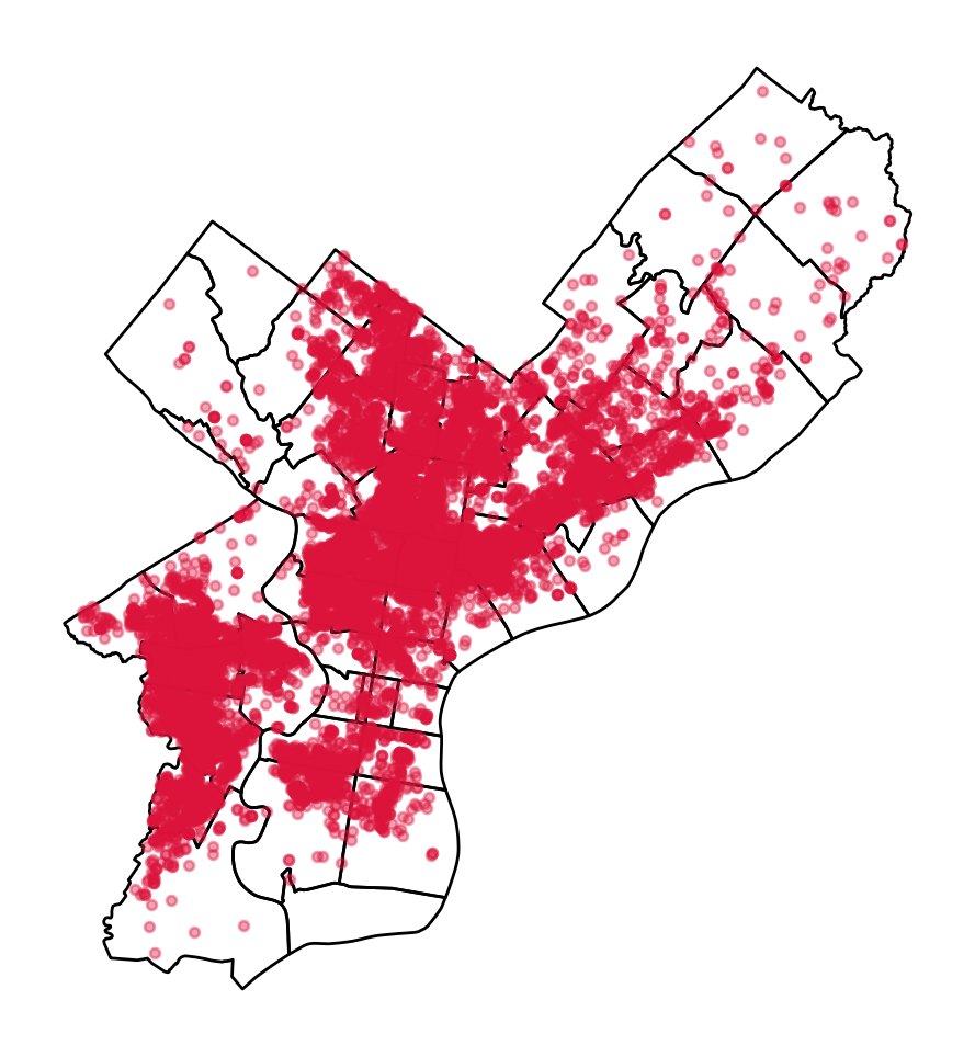

Step 3: Make a (more useful) hex bin map

# Initialize the axes
fig, ax = plt.subplots(figsize=(10, 10), facecolor=plt.get_cmap("viridis")(0))

# Convert to Web Mercator and plot the hexbins
x = shootings.geometry.x
y = shootings.geometry.y
ax.hexbin(x, y, gridsize=40, mincnt=1, cmap="viridis")

# overlay the city limits
zip_codes.to_crs(epsg=3857).plot(
    ax=ax, facecolor="none", linewidth=0.5, edgecolor="white"
)

ax.set_axis_off()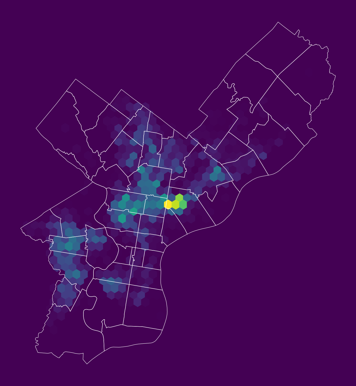

Example: Count the total number of rows in a table

The SQL COUNT function can be applied to count all rows.

response = requests.get(
    carto_api_endpoint, params={"q": "SELECT COUNT(*) FROM shootings"}
)

response.json()

{'rows': [{'count': 15096}],
 'time': 0.006,
 'fields': {'count': {'type': 'number', 'pgtype': 'int8'}},
 'total_rows': 1}

Tip

It’s always a good idea to check how many rows you might be downloading before requesting all of the data from an API!

Example: Select all columns, limiting the total number returned

The LIMIT function limits the number of returned rows. It is very useful for taking a quick look at the format of a database.

# Limit the returned data to only 1 row
query = "SELECT * FROM shootings LIMIT 1"

# Make the request
params = {"q": query, "format": "geojson"}
response = requests.get(carto_api_endpoint, params=params)

Create the GeoDataFrame:

df = gpd.GeoDataFrame.from_features(response.json(), crs="EPSG:4326")

df

	geometry	cartodb_id	objectid	year	dc_key	code	date_	time	race	sex	age	wound	officer_involved	offender_injured	offender_deceased	location	latino	point_x	point_y	dist	inside	outside	fatal
0	POINT (-75.16227 39.98871)	1	10797984	2020	202022062735.0	411	2020-09-12T00:00:00Z	21:04:00	W	M	53	Foot	N	N	N	18TH & DAUPHIN ST	1	-75.162274	39.988715	22	0	1	0

Example: Select by specific column values

Use the WHERE function to select a subset where the logical condition is true.

Example #1: Select nonfatal shootings only

# Select nonfatal shootings only
query = "SELECT * FROM shootings WHERE fatal = 0"

# Make the request
params = {"q": query, "format": "geojson"}
response = requests.get(carto_api_endpoint, params=params)

# Make the GeoDataFrame
nonfatal = gpd.GeoDataFrame.from_features(response.json(), crs="EPSG:4326")

# Print
print("number of nonfatal shootings = ", len(nonfatal))

number of nonfatal shootings =  11878

Example #2: Select shootings in 2023

# Select based on "date_"
query = "SELECT * FROM shootings WHERE date_ >= '1/1/23'"

# Make the request
params = {"q": query, "format": "geojson"}
response = requests.get(carto_api_endpoint, params=params)

# Make the GeoDataFrame
shootings_2023 = gpd.GeoDataFrame.from_features(response.json(), crs="EPSG:4326")

# Print
print("number of shootings in 2023 = ", len(shootings_2023))

number of shootings in 2023 =  1413

At-Home Exercise: Explore trends by month and day of week

Step 1: Convert the date column to `DateTime` objects

Add Month and Day of Week columns

# Condddvert the data column to a datetime object
shootings["date"] = pd.to_datetime(shootings["date_"])

# Add new columns: Month and Day of Week
shootings["Month"] = shootings["date"].dt.month
shootings["Day of Week"] = shootings["date"].dt.dayofweek  # Monday is 0, Sunday is 6

Step 2: Calculate number of shootings by month and day of week

Use the familiar Groupby –> size()

count = shootings.groupby(["Month", "Day of Week"]).size()
count = count.reset_index(name="Count")
count.head()

	Month	Day of Week	Count
0	1	0	168
1	1	1	157
2	1	2	143
3	1	3	139
4	1	4	143

Step 3: Make a heatmap using `hvplot`

# Remember 0 is Monday and 6 is Sunday
count.hvplot.heatmap(
    x="Day of Week",
    y="Month",
    C="Count",
    cmap="viridis",
    width=400,
    height=500,
    flip_yaxis=True,
)

Trends: more shootings on the weekends and in the summer months

Example #3: GeoServices

A GeoService is a standardized format for returning GeoJSON files over the web

Originally developed by Esri, in 2010 the specification was transferred to the Open Web Foundation.

Documentation: http://geoservices.github.io/

Example: Philadelphia neighborhoods

OpenDataPhilly provides GeoService API endpoints for the geometry hosted on its platform

https://opendataphilly.org/datasets/philadelphia-neighborhoods/

# The base URL for the neighborhoods layer
neighborhood_url = "https://services1.arcgis.com/a6oRSxEw6eIY5Zfb/arcgis/rest/services/Philadelphia_Neighborhoods/FeatureServer/0"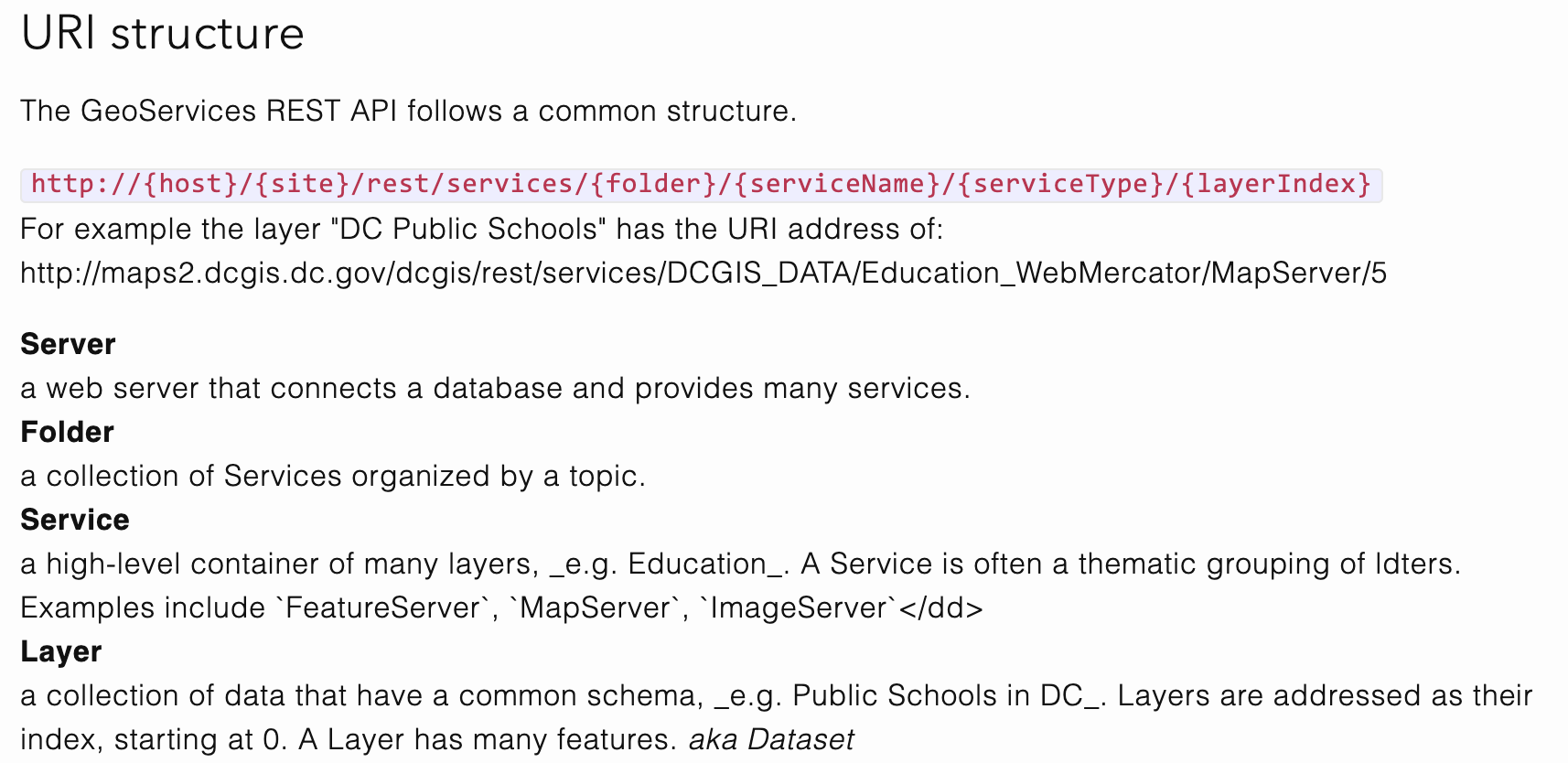

Source: https://geoservices.github.io/resources.html

The `query/` endpoint

Layers have a single endpoint for requesting features: the /query endpoint.

neighborhood_query_endpoint = neighborhood_url + "/query"

neighborhood_query_endpoint

'https://services1.arcgis.com/a6oRSxEw6eIY5Zfb/arcgis/rest/services/Philadelphia_Neighborhoods/FeatureServer/0/query'

The allowed parameters

The main request parameters are:

where: A SQL-like string to select a subset of features; to get all data, use 1=1 (always True)
outFields: The list of columns to return; to get all, use *
f: The returned format; for GeoJSON, use “geojson”
outSR: The desired output CRS

params = {
    "where": "1=1",  # Give me all rows
    "outFields": "*",  # All fields
    "f": "geojson",  # GeoJSON format
    "outSR": "4326",  # The desired output CRS
}

Make the request:

r = requests.get(neighborhood_query_endpoint, params=params)

Get the features and create the GeoDataFrame:

json = r.json()

features = json["features"]

hoods = gpd.GeoDataFrame.from_features(features, crs="EPSG:4326")

hoods

	geometry	FID	NAME	LISTNAME	MAPNAME	Shape_Leng	Shape__Area	Shape__Length
0	POLYGON ((-75.06773 40.00540, -75.06765 40.005...	1	BRIDESBURG	Bridesburg	Bridesburg	27814.546521	7.066581e+06	11074.587308
1	POLYGON ((-75.01560 40.09487, -75.01768 40.092...	2	BUSTLETON	Bustleton	Bustleton	48868.458365	1.812721e+07	19485.686530
2	POLYGON ((-75.18848 40.07273, -75.18846 40.072...	3	CEDARBROOK	Cedarbrook	Cedarbrook	20021.415802	3.950980e+06	7980.051802
3	POLYGON ((-75.21221 40.08603, -75.21211 40.086...	4	CHESTNUT_HILL	Chestnut Hill	Chestnut Hill	56394.297195	1.265385e+07	22476.270236
4	POLYGON ((-75.18479 40.02837, -75.18426 40.027...	5	EAST_FALLS	East Falls	East Falls	27400.776417	6.434879e+06	10907.970158
...	...	...	...	...	...	...	...	...
153	POLYGON ((-75.18373 39.91351, -75.18194 39.913...	154	PACKER_PARK	Packer Park	Packer Park	21816.017948	4.584862e+06	8444.679631
154	POLYGON ((-75.14654 39.93005, -75.14804 39.921...	155	PENNSPORT	Pennsport	Pennsport	11823.233108	1.026917e+06	4706.597865
155	POLYGON ((-75.16986 39.92312, -75.17015 39.921...	156	NEWBOLD	Newbold	Newbold	10052.570885	9.281435e+05	3994.098029
156	POLYGON ((-75.17630 39.92425, -75.17798 39.923...	157	WEST_PASSYUNK	West Passyunk	West Passyunk	10499.291848	1.027608e+06	4173.301421
157	POLYGON ((-75.15684 39.92897, -75.15712 39.927...	158	EAST_PASSYUNK	East Passyunk	East Passyunk	10987.761846	1.028395e+06	4368.384350

158 rows × 8 columns

Now let’s select data just for East Falls and subset the returned columns:

params = {
    "where": "LISTNAME = 'East Falls'",
    "outFields": ["LISTNAME"],
    "f": "geojson",
    "outSR": "4326",
}

r = requests.get(neighborhood_query_endpoint, params=params)

east_falls = gpd.GeoDataFrame.from_features(r.json()["features"], crs="EPSG:4326")

east_falls

	geometry	LISTNAME
0	POLYGON ((-75.18479 40.02837, -75.18426 40.027...	East Falls

Part 2: Natural Language Processing and the 311 Request API

In part two, we’ll pull data using the API for the Philly 311 system, available at: https://iframe.publicstuff.com/#?client_id=242

We saw this site previously when we talked about web scraping last week:

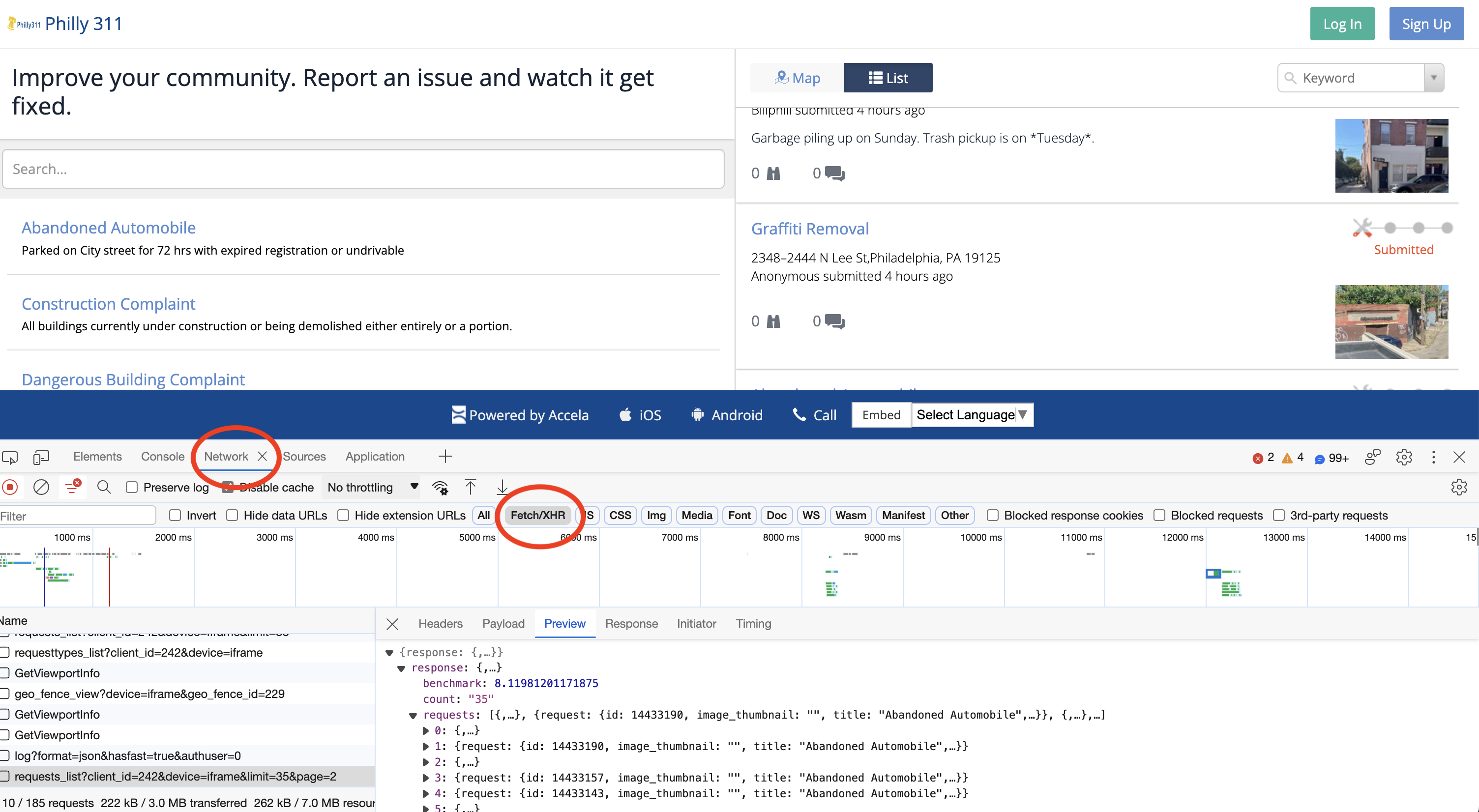
Let’s take another look at the address where the site is pulling its data from:

https://vc0.publicstuff.com/api/2.0/requests_list?client_id=242&device=iframe&limit=35&page=1

This is just an API request! It’s an example of a non-public, internal API, but we can reverse-engineer it to extract the data we want!

Break it down into it’s component parts:

Base URL: https://vc0.publicstuff.com/api/2.0/requests_list
Query parameters: client_id, device, limit, page

It looks likes “client_id” identifies data for the City of Philadelphia, which is definitely a required parameter. Otherwise, the other parameters seem optional, returning the requests on a certain device and viewing page.

Let’s test it out. We’ll grab 2 requests from the first page:

r = requests.get(
    "https://vc0.publicstuff.com/api/2.0/requests_list",
    params={"client_id": 242, "page": 1, "limit": 2},
)

json = r.json()

json

{'response': {'requests': [{'request': {'id': 14500812,
     'image_thumbnail': '',
     'title': 'Traffic Sign Complaint',
     'description': 'People speed up the street like they’re all 95 it needs to have street cushions put in or speed bumps whatever you wanna call',
     'status': 'submitted',
     'address': '3532 Mercer St,Philadelphia, PA 19134',
     'location': 'Philadelphia, Pennsylvania',
     'zipcode': '19134',
     'foreign_id': '16306373',
     'date_created': 1697500549,
     'count_comments': 0,
     'count_followers': 0,
     'count_supporters': 0,
     'lat': 39.98944,
     'lon': -75.095472,
     'user_follows': 0,
     'user_comments': 0,
     'user_request': 0,
     'rank': '1',
     'user': 'Lisa BUCHER'}},
   {'request': {'primary_attachment': {'id': 4618920,
      'extension': 'jpeg',
      'content_type': 'image/jpeg',
      'url': 'https://d17aqltn7cihbm.cloudfront.net/uploads/021404250e358776466e2a1eed0b37b7',
      'versions': {'small': 'https://d17aqltn7cihbm.cloudfront.net/uploads/small_021404250e358776466e2a1eed0b37b7',
       'medium': 'https://d17aqltn7cihbm.cloudfront.net/uploads/medium_021404250e358776466e2a1eed0b37b7',
       'large': 'https://d17aqltn7cihbm.cloudfront.net/uploads/large_021404250e358776466e2a1eed0b37b7'}},
     'id': 14500796,
     'image_thumbnail': 'https://d17aqltn7cihbm.cloudfront.net/uploads/small_021404250e358776466e2a1eed0b37b7',
     'title': 'Abandoned Automobile',
     'description': 'This vehicle has been parked on the 5300 block of Sycamore Street. The car appears to be stolen and parts from the vehicle were removed such as Steering wheel – and other items',
     'status': 'submitted',
     'address': '5414 B St, Philadelphia, PA 19120, USA',
     'location': '',
     'zipcode': None,
     'foreign_id': '16306368',
     'date_created': 1697500317,
     'count_comments': 0,
     'count_followers': 0,
     'count_supporters': 0,
     'lat': 40.0324275675885,
     'lon': -75.1184703964844,
     'user_follows': 0,
     'user_comments': 0,
     'user_request': 0,
     'rank': '1',
     'user': ''}}],
  'count': '2',
  'benchmark': 6.994715929031372,
  'status': {'type': 'success',
   'message': 'Success',
   'code': 200,
   'code_message': 'Ok'}}}

Now we need to understand the structure of the response. First, access the list of requests:

request_list = json["response"]["requests"]

request_list

[{'request': {'id': 14500812,
   'image_thumbnail': '',
   'title': 'Traffic Sign Complaint',
   'description': 'People speed up the street like they’re all 95 it needs to have street cushions put in or speed bumps whatever you wanna call',
   'status': 'submitted',
   'address': '3532 Mercer St,Philadelphia, PA 19134',
   'location': 'Philadelphia, Pennsylvania',
   'zipcode': '19134',
   'foreign_id': '16306373',
   'date_created': 1697500549,
   'count_comments': 0,
   'count_followers': 0,
   'count_supporters': 0,
   'lat': 39.98944,
   'lon': -75.095472,
   'user_follows': 0,
   'user_comments': 0,
   'user_request': 0,
   'rank': '1',
   'user': 'Lisa BUCHER'}},
 {'request': {'primary_attachment': {'id': 4618920,
    'extension': 'jpeg',
    'content_type': 'image/jpeg',
    'url': 'https://d17aqltn7cihbm.cloudfront.net/uploads/021404250e358776466e2a1eed0b37b7',
    'versions': {'small': 'https://d17aqltn7cihbm.cloudfront.net/uploads/small_021404250e358776466e2a1eed0b37b7',
     'medium': 'https://d17aqltn7cihbm.cloudfront.net/uploads/medium_021404250e358776466e2a1eed0b37b7',
     'large': 'https://d17aqltn7cihbm.cloudfront.net/uploads/large_021404250e358776466e2a1eed0b37b7'}},
   'id': 14500796,
   'image_thumbnail': 'https://d17aqltn7cihbm.cloudfront.net/uploads/small_021404250e358776466e2a1eed0b37b7',
   'title': 'Abandoned Automobile',
   'description': 'This vehicle has been parked on the 5300 block of Sycamore Street. The car appears to be stolen and parts from the vehicle were removed such as Steering wheel – and other items',
   'status': 'submitted',
   'address': '5414 B St, Philadelphia, PA 19120, USA',
   'location': '',
   'zipcode': None,
   'foreign_id': '16306368',
   'date_created': 1697500317,
   'count_comments': 0,
   'count_followers': 0,
   'count_supporters': 0,
   'lat': 40.0324275675885,
   'lon': -75.1184703964844,
   'user_follows': 0,
   'user_comments': 0,
   'user_request': 0,
   'rank': '1',
   'user': ''}}]

We need to extract out the “request” key of each list entry. Let’s do that and create a DataFrame:

data = pd.DataFrame([r["request"] for r in request_list])

data.head()

	id	image_thumbnail	title	description	status	address	location	zipcode	foreign_id	date_created	count_comments	count_followers	count_supporters	lat	lon	user_follows	user_comments	user_request	rank	user	primary_attachment
0	14500812		Traffic Sign Complaint	People speed up the street like they’re all 95...	submitted	3532 Mercer St,Philadelphia, PA 19134	Philadelphia, Pennsylvania	19134	16306373	1697500549	0	0	0	39.989440	-75.095472	0	0	0	1	Lisa BUCHER	NaN
1	14500796	https://d17aqltn7cihbm.cloudfront.net/uploads/...	Abandoned Automobile	This vehicle has been parked on the 5300 block...	submitted	5414 B St, Philadelphia, PA 19120, USA		None	16306368	1697500317	0	0	0	40.032428	-75.118470	0	0	0	1		{'id': 4618920, 'extension': 'jpeg', 'content_...

Success! But we want to build up a larger dataset…let’s pull data for the first 3 pages of data. This will take a minute or two…

# Store the data we request
data = []

# Total number of pages
total_pages = 3

# Loop over each page
for page_num in range(1, total_pages + 1):
    # Print out the page number
    print(f"Getting data for page #{page_num}...")

    # Make the request
    r = requests.get(
        "https://vc0.publicstuff.com/api/2.0/requests_list",
        params={
            "client_id": 242,  # Unique identifier for Philadelphia
            "page": page_num,  # What page of data to pull
            "limit": 200,  # How many rows per page
        },
    )

    # Get the json
    d = r.json()

    # Add the new data to our list and save
    data = data + [r["request"] for r in d["response"]["requests"]]

# Create a dataframe
data = pd.DataFrame(data)

Getting data for page #1...
Getting data for page #2...
Getting data for page #3...

len(data)

data.head()

	primary_attachment	id	image_thumbnail	title	description	status	address	zipcode	foreign_id	date_created	lat	lon	rank	user
0	{'id': 4619003, 'extension': 'jpg', 'content_t...	14500990	https://d17aqltn7cihbm.cloudfront.net/uploads/...	Graffiti Removal	On the side of the house, the side facing Wood...	submitted	1320 S Markoe St, Philadelphia, PA 19143, USA	None	16306421	1697503690	39.943466	-75.209642	1	WalkAbout
1	NaN	14500986		Homeless Encampment	There is a growing encampment near my house. T...	submitted	2037 S Broad St, Philadelphia, PA 19148, USA	None	16306417	1697503541	39.924470	-75.169041	1	jimmy.qaqish
2	{'id': 4618993, 'extension': 'jpg', 'content_t...	14500969	https://d17aqltn7cihbm.cloudfront.net/uploads/...	Graffiti Removal	On the west side of S. Markoe Street across fr...	submitted	1305 S Markoe St, Philadelphia, PA 19143, USA	None	16306412	1697503108	39.943874	-75.209812	1	WalkAbout
3	NaN	14500967		Abandoned Automobile	The trailer has been parked on the corner sinc...	submitted	2535 E Ontario St, Philadelphia, PA 19134, USA	None	16306411	1697503064	39.988810	-75.099584	1	cebonfan
4	NaN	14500963		Abandoned Automobile	Parked on the sidewalk for over 6 months	submitted	2634 Sears St, Philadelphia, PA 19146, USA	None	16306410	1697502982	39.936311	-75.188364	1

Let’s focus on the “description” column. This is the narrative text that the user inputs when entering a 311 request, and it is an example of semi-structured data. For the rest of today, we’ll focus on how to extract information from semi-structured data.

Semi-structured data

Data that contains some elements that cannot be easily consumed by computers

Examples: human-readable text, audio, images, etc

Key challenges

Text mining: analyzing blocks of text to extract the relevant pieces of information
Natural language processing (NLP): programming computers to process and analyze human languages
Sentiment analysis: analyzing blocks of text to derive the attitude or emotional state of the person

Note

Twitter is one of the main API examples of semi-structured data, but since Elon Musk overhauled the API access, it’s become prohibitively expensive to access (RIP 💀)

To get started, let’s remove any requests where the description is missing:

data = data.dropna(subset=["description"])
data_final = data.loc[data["description"] != ""]

# Strip out spaces and convert to a list
descriptions = data_final["description"].str.strip().tolist()

descriptions[:10]

['On the side of the house, the side facing Woodland Avenue.',
 'There is a growing encampment near my house. The people there have broken into a fenced area. They are yelling, leaving trash, defecating, and attempting to open cars on the street.',
 'On the west side of S. Markoe Street across from #1305.',
 'The trailer has been parked on the corner since the summer and has not moved. The street facing tires are flat. The trailer seems abandoned.',
 'Parked on the sidewalk for over 6 months',
 'The street light in front of 8219 Fayette st was out last night and is still out tonight. It very, very dark!',
 'On the southwest corner of the intersection of S. 46th Street and Woodland Avenue.',
 "On the 'No Dumping' street sign on the south side of Cedar Avenue about 11 steps west of S. 46th Street. Next to the tiny park.",
 'Apartment complex is dumping trash on our street again! Please help or tell me the proper channels I need to take. Thank you!',
 'People speed up the street like they’re all 95 it needs to have street cushions put in or speed bumps whatever you wanna call']

Use case #1: calculating word frequencies

An example of text mining

Text mining and dealing with messy data

Some steps to clean up our text data:

Break strings into words
Remove capitalization
Remove stop words
Remove punctuation

1. Break strings into words

Use the .split() command to break a string into words by splitting on spaces.

example_string = "This is an Example"

example_string.split()

['This', 'is', 'an', 'Example']

descriptions_words = [desc.split() for desc in descriptions]

descriptions_words[0]

['On',
 'the',
 'side',
 'of',
 'the',
 'house,',
 'the',
 'side',
 'facing',
 'Woodland',
 'Avenue.']

This is a list of lists, e.g., the first element is a list of words. Let’s flatten this into a list of just words:

descriptions_words_flat = []

for list_of_words in descriptions_words:
    for word in list_of_words:
        descriptions_words_flat.append(word)

descriptions_words_flat[0]

'On'

len(descriptions_words_flat)

2. Convert all words to lower case

Use .lower() makes all words lower cased

descriptions_words_lower = [word.lower() for word in descriptions_words_flat]

descriptions_words_lower[:10]

['on',
 'the',
 'side',
 'of',
 'the',
 'house,',
 'the',
 'side',
 'facing',
 'woodland']

len(descriptions_words_lower)

3. Remove stop words

Common words that do not carry much significance and are often ignored in text analysis.

We can use the nltk package.

The “Natural Language Toolkit” https://www.nltk.org/

Import and download the stop words:

import nltk

nltk.download("stopwords");

[nltk_data] Downloading package stopwords to /Users/nhand/nltk_data...
[nltk_data]   Package stopwords is already up-to-date!

Get the list of common stop words:

stop_words = list(set(nltk.corpus.stopwords.words("english")))

stop_words[:10]

["wasn't",
 'will',
 'for',
 'ourselves',
 'while',
 'during',
 'your',
 'here',
 'some',
 "that'll"]

len(stop_words)

descriptions_no_stop = []

for word in descriptions_words_lower:
    if word not in stop_words:
        descriptions_no_stop.append(word)

descriptions_no_stop = [
    word for word in descriptions_words_lower if word not in stop_words
]

len(descriptions_no_stop)

4. Remove punctuation

Get the list of common punctuation:

import string

punctuation = list(string.punctuation)

punctuation[:5]

['!', '"', '#', '$', '%']

Remove punctuation from words:

descriptions_final = []

# Loop over all words
for word in descriptions_no_stop:
    # Remove any punctuation from the words
    for p in punctuation:
        word = word.replace(p, "")

    # Save it if the string is not empty
    if word != "":
        descriptions_final.append(word)

Convert to a Dataframe with one column:

words = pd.DataFrame({"words": descriptions_final})

words.head()

	words
0	side
1	house
2	side
3	facing
4	woodland

Calculate the word frequencies

Use a pandas groupby and sort to put in descending order:

N = (
    words.groupby("words", as_index=False)
    .size()
    .sort_values("size", ascending=False, ignore_index=True)
)

The top 15 words by frequency:

top15 = N.head(15)

top15

	words	size
0	street	145
1	trash	113
2	side	66
3	block	40
4	vehicle	39
5	sidewalk	38
6	please	38
7	property	35
8	lot	35
9	corner	34
10	car	32
11	front	31
12	graffiti	30
13	months	30
14	st	29

Plot the frequencies

Use seaborn to plot our DataFrame of word counts…

fig, ax = plt.subplots(figsize=(8, 8))

# Plot horizontal bar graph
sns.barplot(
    y="words",
    x="size",
    data=top15,
    ax=ax,
    color="#cc3000",
    saturation=1.0,
)

ax.set_title("Most Common Words Found in 311 Requests", fontsize=16);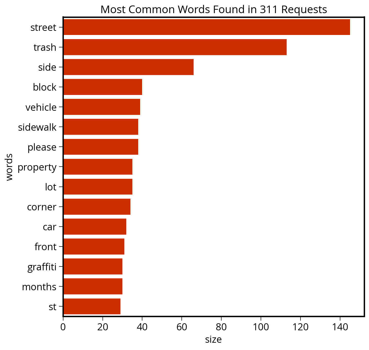

Takeaway: Philly cares about trash! They don’t call it Filthadelphia for nothing…

To be continued next time!

See you on Wednesday!

Part 1: Introduction to APIs

Example #1: Automated data feeds

USGS real-time earthquake feeds

Example #2: The CARTO API

The anatomy of an API request

Let’s try it out in Python

At-Home Exercise: Visualizing shootings data

Example: Count the total number of rows in a table

Example: Select all columns, limiting the total number returned

Example: Select by specific column values

At-Home Exercise: Explore trends by month and day of week

Step 1: Convert the date column to DateTime objects

Step 2: Calculate number of shootings by month and day of week

Step 3: Make a heatmap using hvplot

Example #3: GeoServices

Example: Philadelphia neighborhoods

The query/ endpoint

The allowed parameters

Part 2: Natural Language Processing and the 311 Request API

Semi-structured data

Key challenges

Use case #1: calculating word frequencies

Text mining and dealing with messy data

To be continued next time!

Step 1: Convert the date column to `DateTime` objects

Step 3: Make a heatmap using `hvplot`

The `query/` endpoint