Week 8
Analyzing and Visualizing Large Datasets

Oct 23, 2023
Section 401

This week’s agenda: working with big data

By example: - Open Street Map data - Census data - NYC taxi cab trips

# Initial imports
import matplotlib.pyplot as plt
import numpy as np
import pandas as pd
import geopandas as gpd

The holoViz ecosystem (revisited)

3 new packages: - Dask: analyzing large datasets - Intake: loading data sets into Python - Datashader: visualizing large data sets

First up: dask

Out-of-core (larger-than-memory) operations in Python

Extends the maximum file size from the size of memory to the size of your hard drive

The key: lazy evaluation

Dask stores does not evaluate expressions immediately — rather it stores a task graph of the necessary calculations.

Numpy arrays

# Create an array of normally-distributed random numbers
a = np.random.randn(1000)

a[:10]

array([ 1.19762135,  1.83169553,  1.70239442,  1.5931158 , -1.42665936,
       -0.58410114, -0.95528754, -0.62491725,  1.35811674, -1.47935545])

# Multiply this array by a factor
b = a * 4

# Find the minimum value
b_min = b.min()


b_min

-11.875423971838202

Dask arrays mirror the numpy array syntax…but don’t perform the calculation right away.

import dask.array as da

# Create a dask array from the above array
a_dask = da.from_array(a, chunks=200)

# Multiply this array by a factor
b_dask = a_dask * 4

# Find the minimum value
b_min_dask = b_dask.min()

print(b_min_dask)

dask.array<amin-aggregate, shape=(), dtype=float64, chunksize=(), chunktype=numpy.ndarray>

We need to explicitly call the compute() function to evaluate the expression. We get the same result as the non-lazy numpy result.

b_min_dask.compute()

-11.875423971838202

Dask dataframes

Syntax mirrors the Pandas DataFrame object
Uses the task graph functionality to provides a unified interface to multiple pandas DataFrame objects.

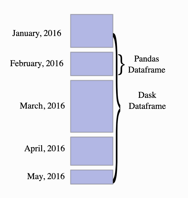
Enables out-of-core operations

Pandas DataFrames don’t need to fit into memory…when evaluating an expression, dask will load the data into memory when necessary.

Let’s try it out:

Loading 1 billion Open Street Map points…

Source

Loading data with intake

Intake helps make loading data into Python very easy
Works with the holoViz ecosystem, including dask
We’ll load the OSM data from Amazon s3:
- http://s3.amazonaws.com/datashader-data/osm-1billion.snappy.parq.zip

An intake “catalog”

Metadata that tells Python where and how to download data
On first download, the data is cached locally to avoid repeated downloaded
Creates a standard way of sharing datasets

See datasets.yml in this week’s repository.

Load our intake catalog

import intake

datasets = intake.open_catalog("./datasets.yml")

Which datasets do we have?

list(datasets)

['nyc_taxi_wide', 'census', 'osm']

3 “big data” examples today

1 billion OSM points: http://s3.amazonaws.com/datashader-data/osm-1billion.parq.zip
NYC taxi trips: https://s3.amazonaws.com/datashader-data/nyc_taxi_wide.parq
2010 Census data: http://s3.amazonaws.com/datashader-data/census2010.parq.zip

Example 1: OSM data points

Convert the data to a dask array: `to_dask()`

This step downloads the data.
The first time you run it, you should see a progress bar documenting the download progress.
Given the size of the data files (> 1 GB), the download can take several minutes.

type(datasets.osm)

intake_parquet.source.ParquetSource

osm_ddf = datasets.osm.to_dask()

osm_ddf

Dask DataFrame Structure:

	x	y
npartitions=119
	float32	float32
	...	...
...	...	...
	...	...
	...	...

Dask Name: read-parquet, 1 graph layer

Remember

The data frame is sub-divided into 119 partitions and only one partition will be loaded into memory at a time.
No actual data has been loaded from the file yet!

Let’s load the data for the first partition to peek at the head of the file

Only the data necessary to see the head of the file will be loaded.

# we can still get the head of the file quickly
osm_ddf.head(n=10)

	x	y
0	-16274360.0	-17538778.0
1	-16408889.0	-16618700.0
2	-16246231.0	-16106805.0
3	-19098164.0	-14783157.0
4	-17811662.0	-13948767.0
5	-17751736.0	-13926740.0
6	-17711376.0	-13921245.0
7	-17532738.0	-13348323.0
8	-19093358.0	-10380358.0
9	-19077458.0	-10445329.0

Note: What geographic coordinates?

Data is in Web Mercator (EPSG=3857) coordinates
Units are meters

How about the size of the data frame?

All data partitions must be loaded for this calculation…it will take longer!

# getting the length means all of the data must be loaded though
nrows = len(osm_ddf)
print(f"number of rows = {nrows}")

number of rows = 1000050363

1 billion rows!

Let’s do some simple calculations

# mean x/y coordinates
mean_x = osm_ddf['x'].mean()
mean_y = osm_ddf['y'].mean()

print(mean_x, mean_y)

dd.Scalar<series-..., dtype=float32> dd.Scalar<series-..., dtype=float32>

# evaluate the expressions
print("mean x = ", mean_x.compute())

mean x =  2731828.836864097

# evaluate the expressions
print("mean y = ", mean_y.compute())

mean y =  5801830.125332437

Now let’s visualize the points…but how?

Not with matplotlib…

Matplotlib struggles with only hundreds of points

Enter Datashader

“Turns even the largest data into images, accurately”

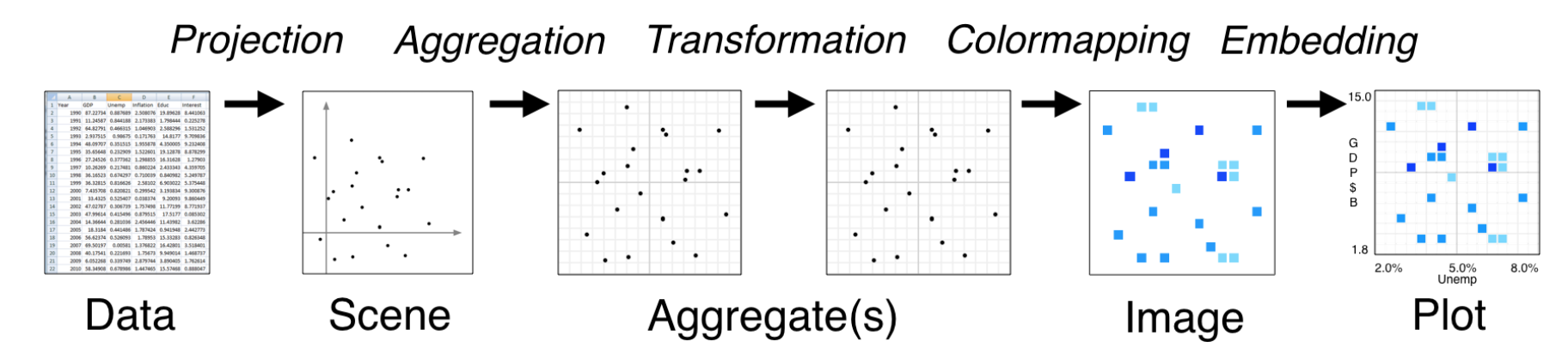
Datashader is a library that produces a “rasterized” image of large datasets, such that the visual color mapping is a fair representation of the underlying data.

The Datashader pipeline

Aggregate data onto a pixelized image
Map aggregated data to colors to properly represent density of data

Recommended reading: Understanding the datashader algorithm

# Datashader imports
import datashader as ds
import datashader.transfer_functions as tf

# Color-related imports
from datashader.colors import Greys9, viridis, inferno
from colorcet import fire

Steps:

Initialize a datashader Canvas() with a specific width & height and x & y ranges (“extent”)
Aggregate the x/y points on the canvas into pixels, using a specified aggregation function

Important

datashader requires Web Mercator coordinates (EPSG=3857)
In this case, the data is already in the right coordinates so no transformation is needed

Set up the global datashader canvas:

# Web Mercator bounds
bound = 20026376.39
global_x_range = (-bound, bound)
global_y_range = (int(-bound*0.4), int(bound*0.6))

# Default width and height
global_plot_width = 900
global_plot_height = int(global_plot_width*0.5)

# Step 1: Setup the canvas
canvas = ds.Canvas(
    plot_width=global_plot_width,
    plot_height=global_plot_height,
    x_range=global_x_range,
    y_range=global_y_range,
)
 
# Step 2: Aggregate the points into pixels
# NOTE: Use the "count()" function — count number of points per pixel
agg = canvas.points(osm_ddf, "x", "y", agg=ds.count())

Note: The aggregated pixels are stored using xarray

agg

Steps (continued)

Perform the “shade” operation — map the pixel values to a color map

# Step 3: Perform the shade operation
img = tf.shade(agg, cmap=fire)

# Format: set the background of the image to black so it looks better
img = tf.set_background(img, "black")

img

Improvement: Remove noise from pixels with low counts

Remember: our agg variable is an xarray DataArray.

So, we can leverage xarray’s builtin where() function to select a subsample of the pixels based on the pixel counts.

selected = agg.where(agg > 15)
selected

This will mask pixels that do not satisfy the `where` condition — masked pixels are set to NaN

# plot the masked data
tf.set_background(tf.shade(selected, cmap=fire),"black")

Example 2: Revisiting the census dot map

We can use datashader to visualize all 300 million census dots to make a nationwide version of the racial dot map we saw in week 7.

# Load the data
# REMEMBER: this will take some time to download the first time
census_ddf = datasets.census.to_dask()

census_ddf

Dask DataFrame Structure:

	easting	northing	race
npartitions=36
	float32	float32	category[unknown]
	...	...	...
...	...	...	...
	...	...	...
	...	...	...

Dask Name: read-parquet, 1 graph layer

census_ddf.head()

	easting	northing	race
0	-12418767.0	3697425.00	h
1	-12418512.0	3697143.50	h
2	-12418245.0	3697584.50	h
3	-12417703.0	3697636.75	w
4	-12418120.0	3697129.25	h

Note: What geographic coordinates?

Once again, data is in Web Mercator (EPSG=3857) coordinates
“easting” is the x coordinate and “northing” is the y coordinate
Units are meters

print("number of rows =", len(census_ddf))

number of rows = 306675004

Roughly 300 million rows: 1 for each person in the U.S. population

Set up bounds for major cities and USA

Important: datashader has a utility function to convert from latitude/longitude (EPSG=4326) to Web Mercator (EPSG=3857)

See: lnglat_to_meters()

from datashader.utils import lnglat_to_meters

# Sensible lat/lng coordinates for U.S. cities
# NOTE: these are in lat/lng so EPSG=4326
USA           = [(-124.72,  -66.95), (23.55, 50.06)]
Chicago       = [( -88.29,  -87.30), (41.57, 42.00)]
NewYorkCity   = [( -74.39,  -73.44), (40.51, 40.91)]
LosAngeles    = [(-118.53, -117.81), (33.63, 33.96)]
Houston       = [( -96.05,  -94.68), (29.45, 30.11)]
Austin        = [( -97.91,  -97.52), (30.17, 30.37)]
NewOrleans    = [( -90.37,  -89.89), (29.82, 30.05)]
Atlanta       = [( -84.88,  -84.04), (33.45, 33.84)]
Philly        = [( -75.28,  -74.96), (39.86, 40.14)]


# Get USA xlim and ylim in meters (EPSG=3857)
USA_xlim_meters, USA_ylim_meters = [list(r) for r in lnglat_to_meters(USA[0], USA[1])]

# Define some a default plot width & height
plot_width  = int(900)
plot_height = int(plot_width*7.0/12)

First, visualize the population density

How about a linear color scale?

# Step 1: Setup the canvas
cvs = ds.Canvas(
    plot_width, plot_height, x_range=USA_xlim_meters, y_range=USA_ylim_meters
)

# Step 2: Aggregate the x/y points
agg = cvs.points(census_ddf, "easting", "northing")

# Step 3: Shade with a "Grey" colormap and "linear" colormapping
img = tf.shade(agg, cmap=Greys9, how="linear")

# Format: Set the background
tf.set_background(img, "black")

Okay, what about a log scale?

# Step 3: Shade with a "Grey" colormap and "log" colormapping
img = tf.shade(agg, cmap=Greys9, how='log')

# Format: add a black background
img = tf.set_background(img, 'black')
img

Let’s use a perceptually uniform color map

“A collection of perceptually accurate colormaps”

See: https://colorcet.holoviz.org/

## Step 3: Shade with "fire" color scale and "log" colormapping
img = tf.shade(agg, cmap=fire, how='log')
tf.set_background(img, 'black')

The best option: using the equal histogram method for shading

This is the default shading option for color mapping in datashader
A common image processing technique for improving contrast and equalizing pixel values across images

# Step 3: Shade with fire colormap and equalized histogram mapping
img = tf.shade(agg, cmap=fire, how='eq_hist')
tf.set_background(img, 'black')

How about viridis?

img = tf.shade(agg, cmap=viridis, how='eq_hist')
img = tf.set_background(img, 'black')
img

How to save?

Use the export_image() function.

from datashader.utils import export_image

export_image(img, 'usa_census_viridis')

Next, let’s visualize race

Datashader can plot use different colors for different categories of data.

census_ddf.head()

	easting	northing	race
0	-12418767.0	3697425.00	h
1	-12418512.0	3697143.50	h
2	-12418245.0	3697584.50	h
3	-12417703.0	3697636.75	w
4	-12418120.0	3697129.25	h

census_ddf['race'].value_counts().compute()

w    196052887
h     50317503
b     37643995
a     13914371
o      8746248
Name: race, dtype: int64

Define a color scale for each race category

color_key = {"w": "aqua", "b": "lime", "a": "red", "h": "fuchsia", "o": "yellow"}

def create_census_image(longitude_range, latitude_range, w=plot_width, h=plot_height):
    """
    A function for plotting the Census data, coloring pixel by race values.
    """
    # Step 1: Calculate x and y range from lng/lat ranges
    x_range, y_range = lnglat_to_meters(longitude_range, latitude_range)

    # Step 2: Setup the canvas
    canvas = ds.Canvas(plot_width=w, plot_height=h, x_range=x_range, y_range=y_range)

    # Step 3: Aggregate, but this time count the "race" category
    # NEW: specify the aggregation method to count the "race" values in each pixel
    agg = canvas.points(census_ddf, "easting", "northing", agg=ds.count_cat("race"))
    
    # Step 4: Shade, using our custom color map
    img = tf.shade(agg, color_key=color_key, how="eq_hist")

    # Return image with black background
    return tf.set_background(img, "black")

Let’s visualize all 300 million points

Color pixel values according to the demographics data in each pixel.

create_census_image(USA[0], USA[1])

Remember: color scheme

White: aqua
Black/African American: lime
Asian: red
Hispanic: fuchsia
Other: yellow

Let’s zoom in on Philadelphia…

create_census_image(Philly[0], Philly[1], w=600, h=600)

At home exercise: what about other cities?

Hint: use the bounding boxes provided earlier to explore racial patterns across various major cities

New York City

create_census_image(NewYorkCity[0], NewYorkCity[1])

Atlanta

create_census_image(Atlanta[0], Atlanta[1])

Los Angeles

create_census_image(LosAngeles[0], LosAngeles[1])

Houston

create_census_image(Houston[0], Houston[1])

Chicago

create_census_image(Chicago[0], Chicago[1])

New Orleans

create_census_image(NewOrleans[0], NewOrleans[1])

Can we learn more than just population density and race?

We can use xarray to slice the array of aggregated pixel values to examine specific aspects of the data.

Question: Where do African Americans live?

Use the sel() function of the xarray array

# Step 1: Setup canvas
cvs = ds.Canvas(plot_width=plot_width, plot_height=plot_height)

# Step 2: Aggregate and count race category
aggc = cvs.points(census_ddf, "easting", "northing", agg=ds.count_cat("race"))

# NEW: Select only African Americans (where "race" column is equal to "b")
agg_b = aggc.sel(race="b")

agg_b

# Step 3: Shade and set background
img = tf.shade(agg_b, cmap=fire, how="eq_hist")
img = tf.set_background(img, "black")

img

Question: How to identify diverse areas?

Goal: Select pixels where each race has a non-zero count.

bool_sel = aggc.sel(race=['w', 'b', 'a', 'h']) > 0

bool_sel

# Do a "logical and" operation across the "race" dimension
# Pixels will be "True" if the pixel has a positive count for each race
diverse_selection = bool_sel.all(dim='race')

diverse_selection

# Select the pixel values where our diverse selection criteria is True
agg2 = aggc.where(diverse_selection).fillna(0)

# and shade using our color key
img = tf.shade(agg2, color_key=color_key, how='eq_hist')
img = tf.set_background(img,"black")

img

Question: Where is African American population greater than the White population?

# Select where the "b" race dimension is greater than the "w" race dimension
selection = aggc.sel(race='b') > aggc.sel(race='w') 

selection

# Select based on the selection criteria
agg3 = aggc.where(selection).fillna(0)

img = tf.shade(agg3, color_key=color_key, how="eq_hist")
img = tf.set_background(img, "black")

img

This week’s agenda: working with big data

The holoViz ecosystem (revisited)

First up: dask

The key: lazy evaluation

Numpy arrays

Dask dataframes

Enables out-of-core operations

Loading data with intake

An intake “catalog”

Load our intake catalog

Which datasets do we have?

3 “big data” examples today

Example 1: OSM data points

Convert the data to a dask array: to_dask()

Let’s load the data for the first partition to peek at the head of the file

Note: What geographic coordinates?

How about the size of the data frame?

Let’s do some simple calculations

Now let’s visualize the points…but how?

Not with matplotlib…

Enter Datashader

The Datashader pipeline

Steps:

Steps (continued)

Improvement: Remove noise from pixels with low counts

This will mask pixels that do not satisfy the where condition — masked pixels are set to NaN

Example 2: Revisiting the census dot map

Note: What geographic coordinates?

Roughly 300 million rows: 1 for each person in the U.S. population

Set up bounds for major cities and USA

First, visualize the population density

The best option: using the equal histogram method for shading

Next, let’s visualize race

Define a color scale for each race category

Let’s visualize all 300 million points

Remember: color scheme

Let’s zoom in on Philadelphia…

At home exercise: what about other cities?

New York City

Atlanta

Los Angeles

Houston

Chicago

New Orleans

Can we learn more than just population density and race?

Question: Where do African Americans live?

Question: How to identify diverse areas?

Question: Where is African American population greater than the White population?

To be continued…

Convert the data to a dask array: `to_dask()`

This will mask pixels that do not satisfy the `where` condition — masked pixels are set to NaN