Week 14: Raster Data in the Wild

Section 401
Dec 6, 2023

from matplotlib import pyplot as plt
import numpy as np
import pandas as pd
import geopandas as gpd

np.seterr("ignore");

Last two lectures!

Raster data analysis with the holoviz ecosystem

Two case studies:

Using satellite imagery to detect changes in lake volume
Detecting urban heat islands in Philadelphia

The decline of the world’s saline lakes

A 2017 study that looked at the volume decline of many of the world’s saline lakes
Primarily due to water diversion and climate change
Estimate the amount of inflow required to sustain these ecosystems
Copy of the study available in this week’s repository

Some examples…

The Aral Sea in Kazakhstan

2000

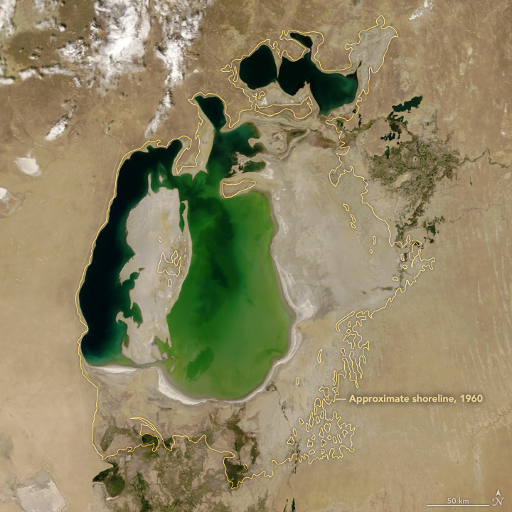
2018

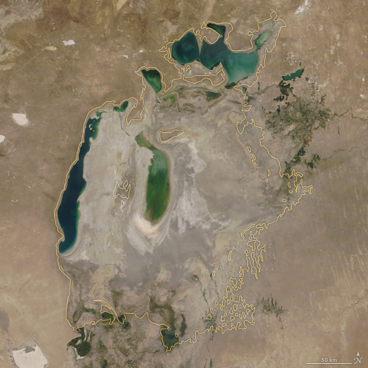
Source: https://earthobservatory.nasa.gov/world-of-change/AralSea

Lake Urmia in Iran

1998

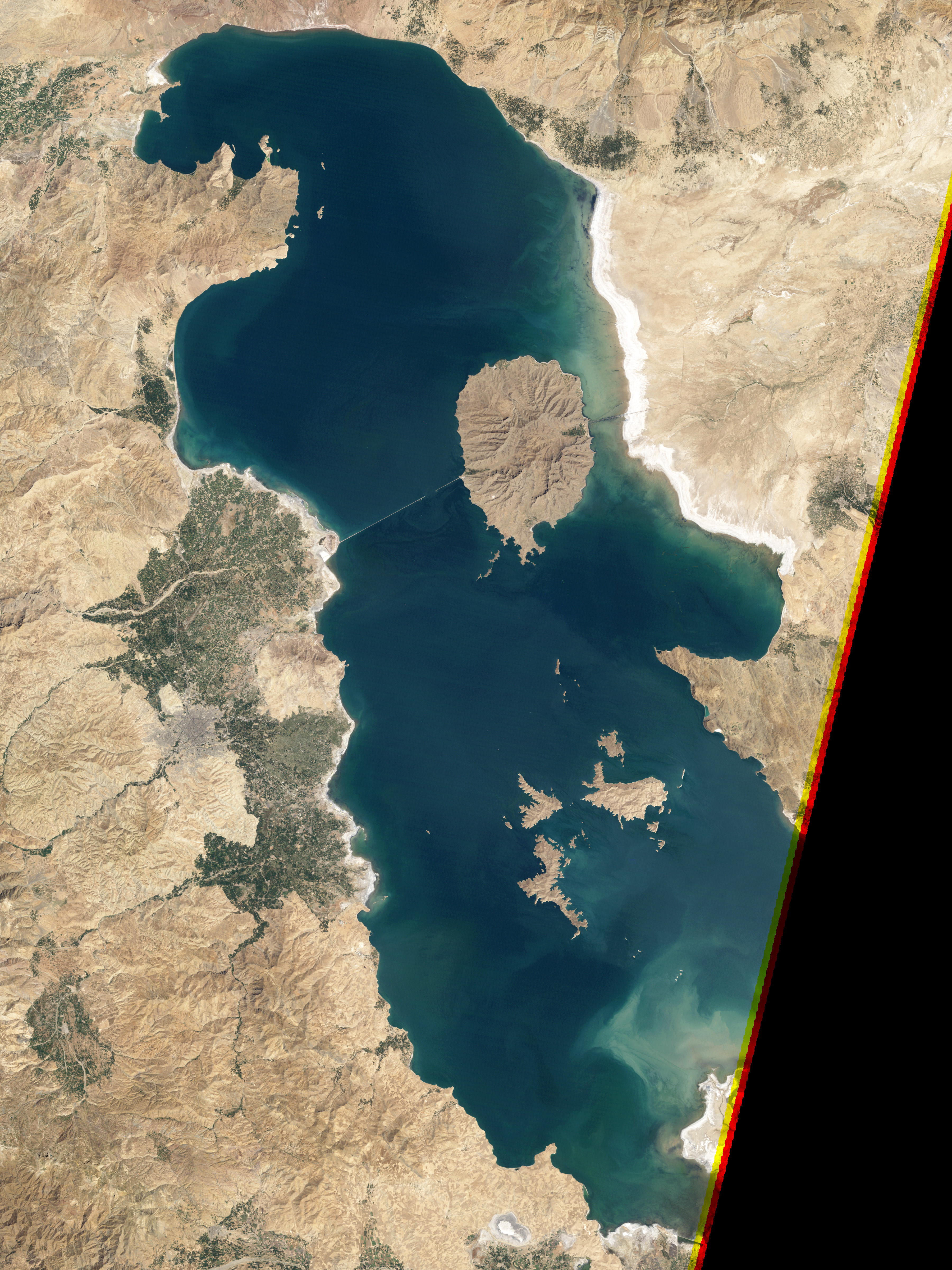
2011

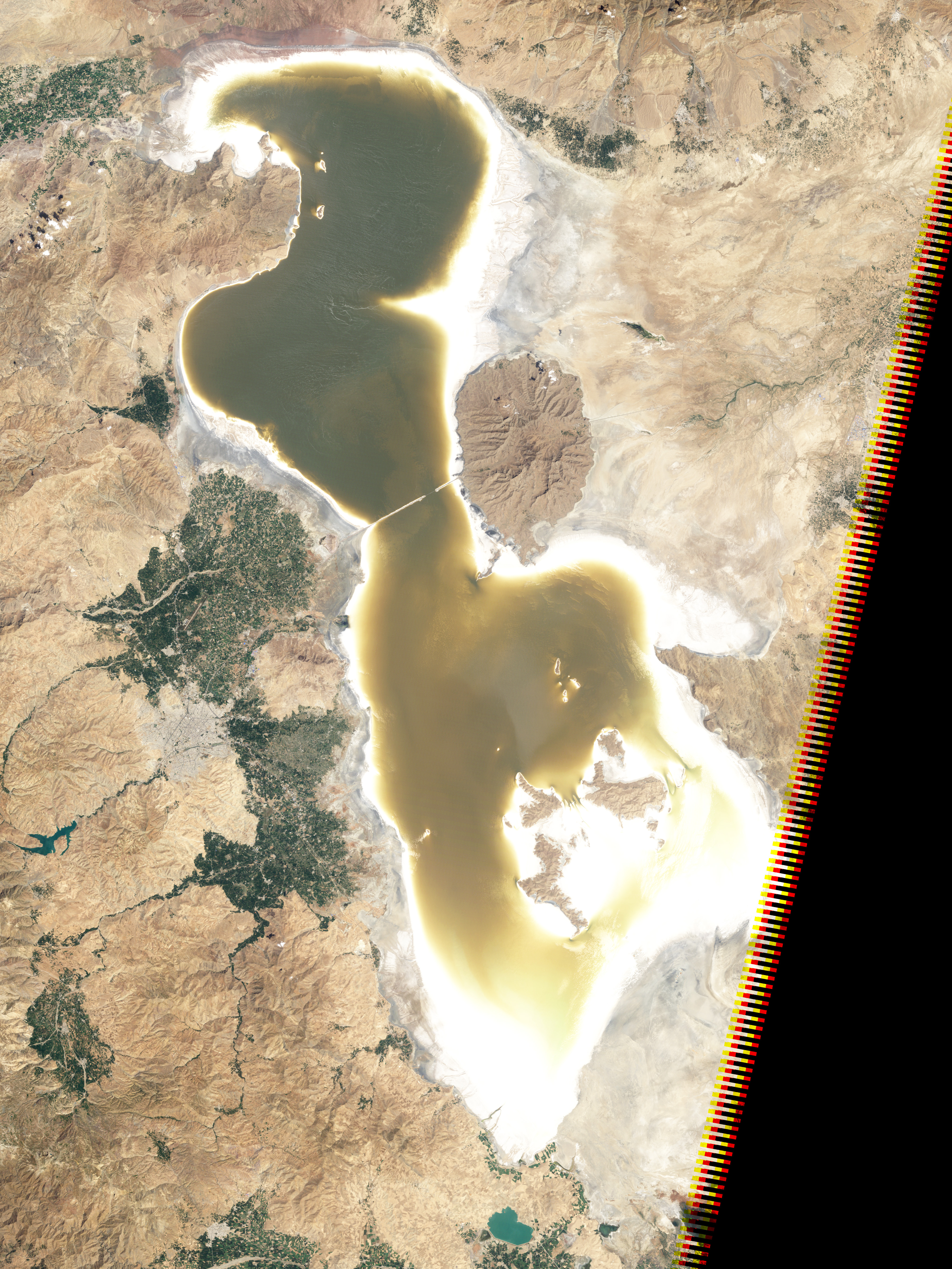
Source: https://earthobservatory.nasa.gov/images/76327/lake-orumiyeh-iran

Today: Walker Lake

1988

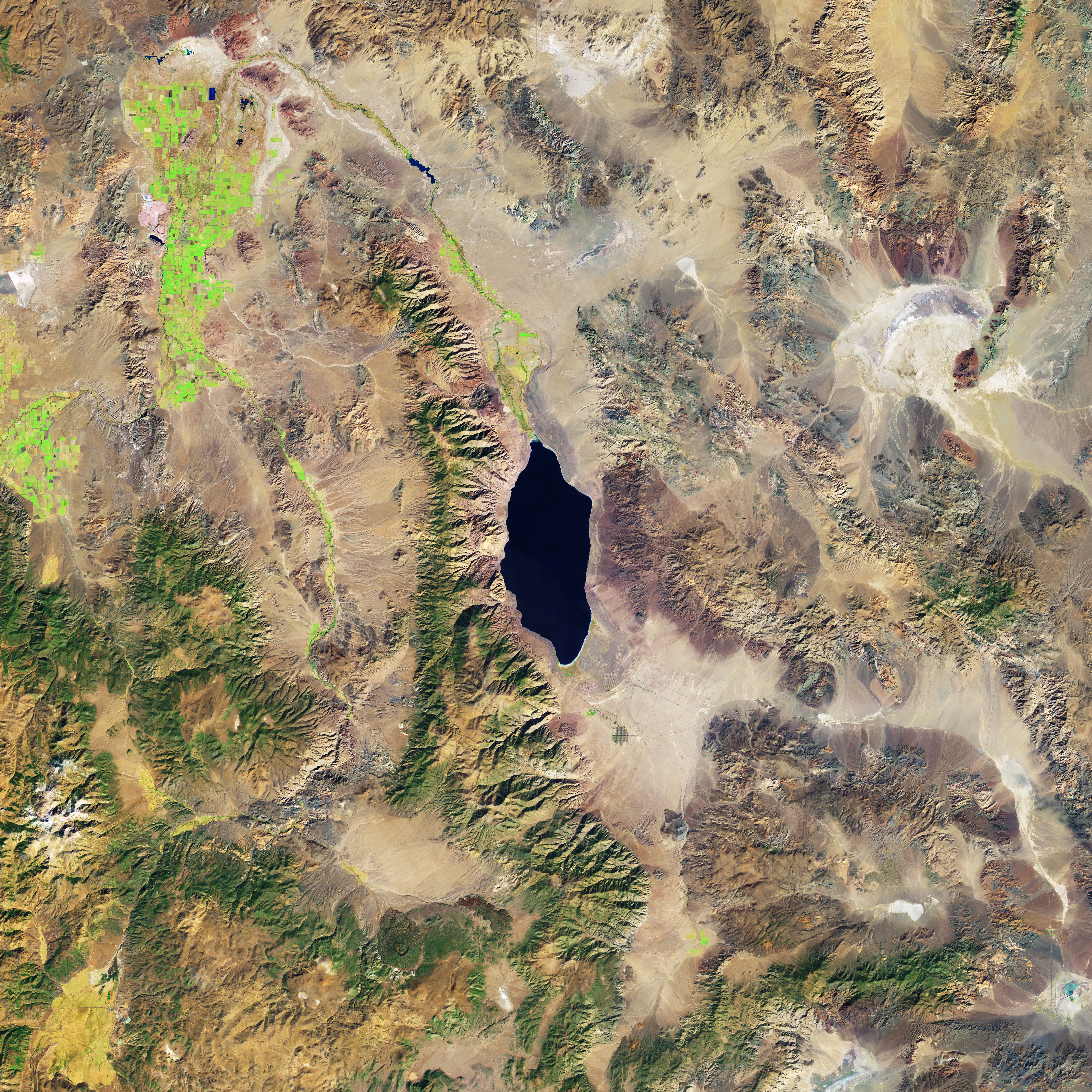
2017

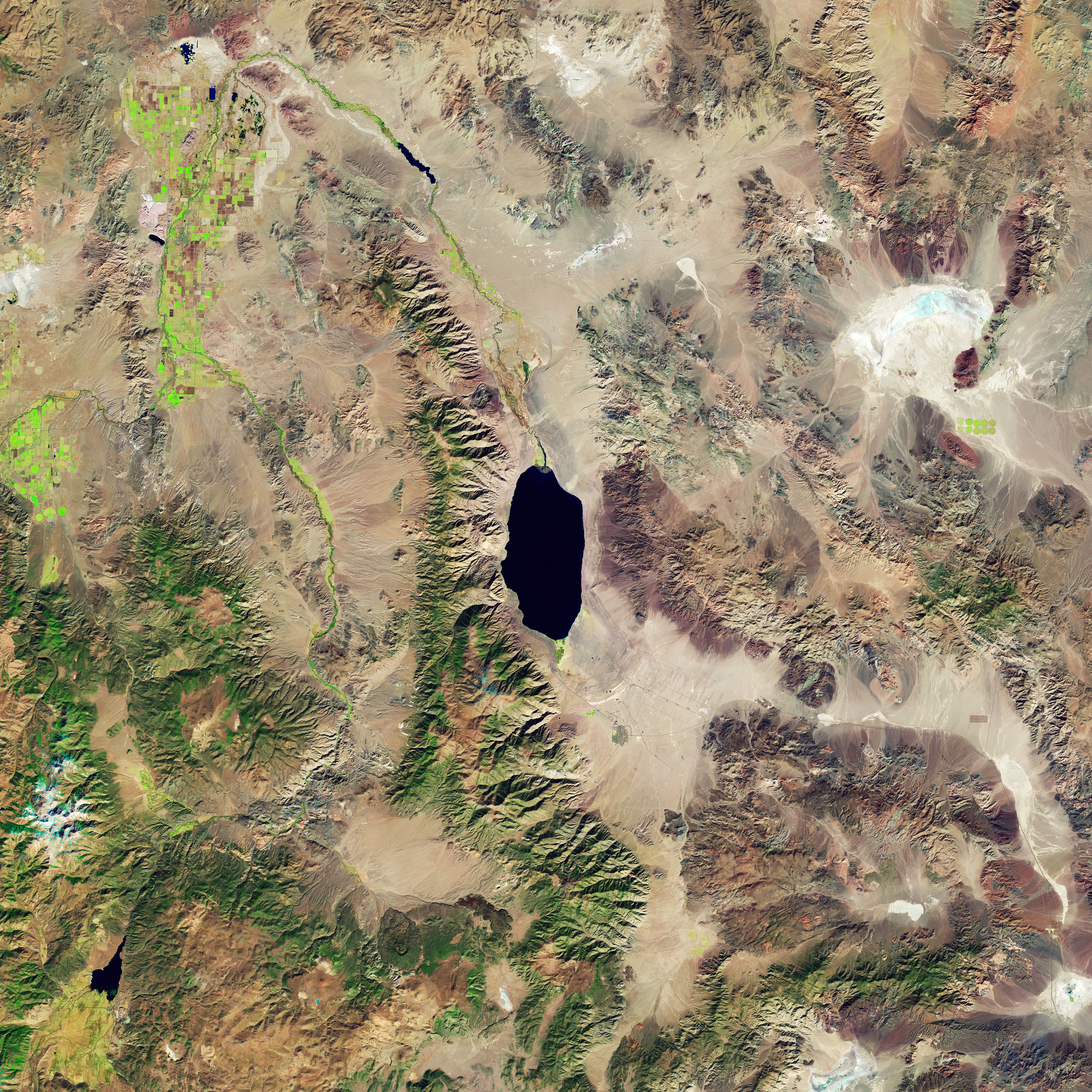
Source: https://earthobservatory.nasa.gov/images/91921/disappearing-walker-lake

Let’s analyze this in Python!

import intake
import xarray as xr

# hvplot
import hvplot.xarray
import hvplot.pandas

import holoviews as hv
import geoviews as gv
from geoviews.tile_sources import EsriImagery

First, let’s use intake to load the data

Catalog file: https://github.com/pyviz-topics/EarthML/blob/master/examples/catalog.yml

Source: EarthML

url = 'https://raw.githubusercontent.com/pyviz-topics/EarthML/master/examples/catalog.yml'
cat = intake.open_catalog(url)

list(cat)

['landsat_5_small',
 'landsat_8_small',
 'landsat_5',
 'landsat_8',
 'google_landsat_band',
 'amazon_landsat_band',
 'fluxnet_daily',
 'fluxnet_metadata',
 'seattle_lidar']

We’ll focus on the Landsat 5 and 8 small datasets.

These are “small” snapshots around Walker Lake, around cut out of the larger Landsat dataset.

landsat_5 = cat.landsat_5_small()

type(landsat_5)

intake_xarray.raster.RasterIOSource

landsat_5

landsat_5_small:
  args:
    chunks:
      band: 1
      x: 50
      y: 50
    concat_dim: band
    storage_options:
      anon: true
    urlpath: s3://earth-data/landsat/small/LT05_L1TP_042033_19881022_20161001_01_T1_sr_band{band:d}.tif
  description: Small version of Landsat 5 Surface Reflectance Level-2 Science Product.
  driver: intake_xarray.raster.RasterIOSource
  metadata:
    cache:
    - argkey: urlpath
      regex: earth-data/landsat
      type: file
    catalog_dir: https://raw.githubusercontent.com/pyviz-topics/EarthML/master/examples
    plots:
      band_image:
        dynamic: false
        groupby: band
        kind: image
        rasterize: true
        width: 400
        x: x
        y: y

Intake let’s you define “default” plots for a dataset

Leveraging the power of hvplot under the hood…

landsat_5.hvplot.band_image()

What’s happening under the hood?

landsat_5.hvplot.image(
    x="x",
    y="y",
    groupby="band",
    rasterize=True,
    frame_width=400,
    frame_height=400,
    geo=True,
    crs=32611,
)

We can do the same for the Landsat 8 data

landsat_8 = cat.landsat_8_small()

landsat_8.hvplot.image(
    x="x",
    y="y",
    groupby="band",
    rasterize=True,
    frame_width=400,
    frame_height=400,
    geo=True,
    crs=32611,
)

We can use dask to read the data

This will return an xarray DataArray where the values are stored as dask arrays.

landsat_5_da = landsat_5.to_dask()
landsat_8_da = landsat_8.to_dask()

landsat_5_da

Use “.values” to convert to a numpy array

landsat_5_da.shape

(6, 300, 300)

landsat_5_da.values

array([[[ 640.,  842.,  864., ..., 1250.,  929., 1111.],
        [ 796.,  774.,  707., ..., 1136.,  906., 1065.],
        [ 975.,  707.,  908., ..., 1386., 1249., 1088.],
        ...,
        [1243., 1202., 1160., ..., 1132., 1067.,  845.],
        [1287., 1334., 1292., ...,  801.,  934.,  845.],
        [1550., 1356., 1314., ..., 1309., 1636., 1199.]],

       [[ 810., 1096., 1191., ..., 1749., 1266., 1411.],
        [1096., 1048.,  905., ..., 1556., 1217., 1411.],
        [1286., 1000., 1286., ..., 1749., 1604., 1411.],
        ...,
        [1752., 1565., 1566., ..., 1502., 1456., 1078.],
        [1752., 1799., 1706., ...,  983., 1172., 1077.],
        [1893., 1753., 1754., ..., 1736., 2250., 1736.]],

       [[1007., 1345., 1471., ..., 2102., 1462., 1719.],
        [1260., 1259., 1175., ..., 1847., 1419., 1719.],
        [1555., 1175., 1555., ..., 2059., 1889., 1760.],
        ...,
        [2090., 1840., 1798., ..., 1828., 1703., 1242.],
        [2048., 2049., 2008., ..., 1074., 1326., 1158.],
        [2216., 1965., 2049., ..., 2202., 2783., 1994.]],

       [[1221., 1662., 1809., ..., 2401., 1660., 1957.],
        [1564., 1465., 1367., ..., 2105., 1610., 1907.],
        [2004., 1465., 1955., ..., 2302., 2055., 2006.],
        ...,
        [2429., 2138., 2041., ..., 2175., 1885., 1301.],
        [2381., 2333., 2382., ..., 1204., 1495., 1301.],
        [2478., 2041., 2333., ..., 2755., 3431., 2223.]],

       [[1819., 2596., 2495., ..., 2429., 1785., 2023.],
        [2259., 2359., 1885., ..., 2158., 1684., 1921.],
        [2865., 2291., 2664., ..., 2057., 1955., 2057.],
        ...,
        [3081., 2679., 2612., ..., 2499., 2098., 1395.],
        [2779., 2544., 2779., ..., 1429., 1596., 1496.],
        [3183., 2309., 2679., ..., 3067., 3802., 2665.]],

       [[1682., 2215., 2070., ..., 2072., 1440., 1780.],
        [1876., 1973., 1633., ..., 1926., 1586., 1635.],
        [2409., 1924., 2215., ..., 1829., 1780., 1829.],
        ...,
        [2585., 2296., 2296., ..., 2093., 1710., 1134.],
        [2393., 2344., 2489., ..., 1182., 1374., 1326.],
        [2826., 2007., 2393., ..., 2860., 3724., 2333.]]])

Important

EPSG 32611 is the default CRS for Landsat data
Units are meters

Evidence of shrinkage?

We want to compare the images across time.
Data for Landsat 8 is from 2017
Data for Landat 5 is from 1988

Problem: they appear to cover different areas

First: Let’s plot RGB images of the two datasets

See lecture 5B for a reminder!

Hints - We want to use the earthpy package to do the plotting. - We can use the data.sel(band=bands) syntax to select specific bands from the dataset, where bands is a list of the desired bands to be selected.

Important notes

For Landsat 5, the RGB bands are bands 3, 2, and 1, respectively.
For Landsat 8, the RGB bands are bands 4, 3, and 2, respectively.
Reference: Landsat 5 and Landsat 8

import earthpy.plot as ep

Landsat 8 color image

# Get the RGB data from landsat 8 dataset as a numpy array
rgb_data_8 = landsat_8_da.sel(band=[4,3,2]).values

# # Initialize
fig, ax = plt.subplots(figsize=(10,10))

# # Plot the RGB bands
ep.plot_rgb(rgb_data_8, rgb=(0, 1, 2), ax=ax);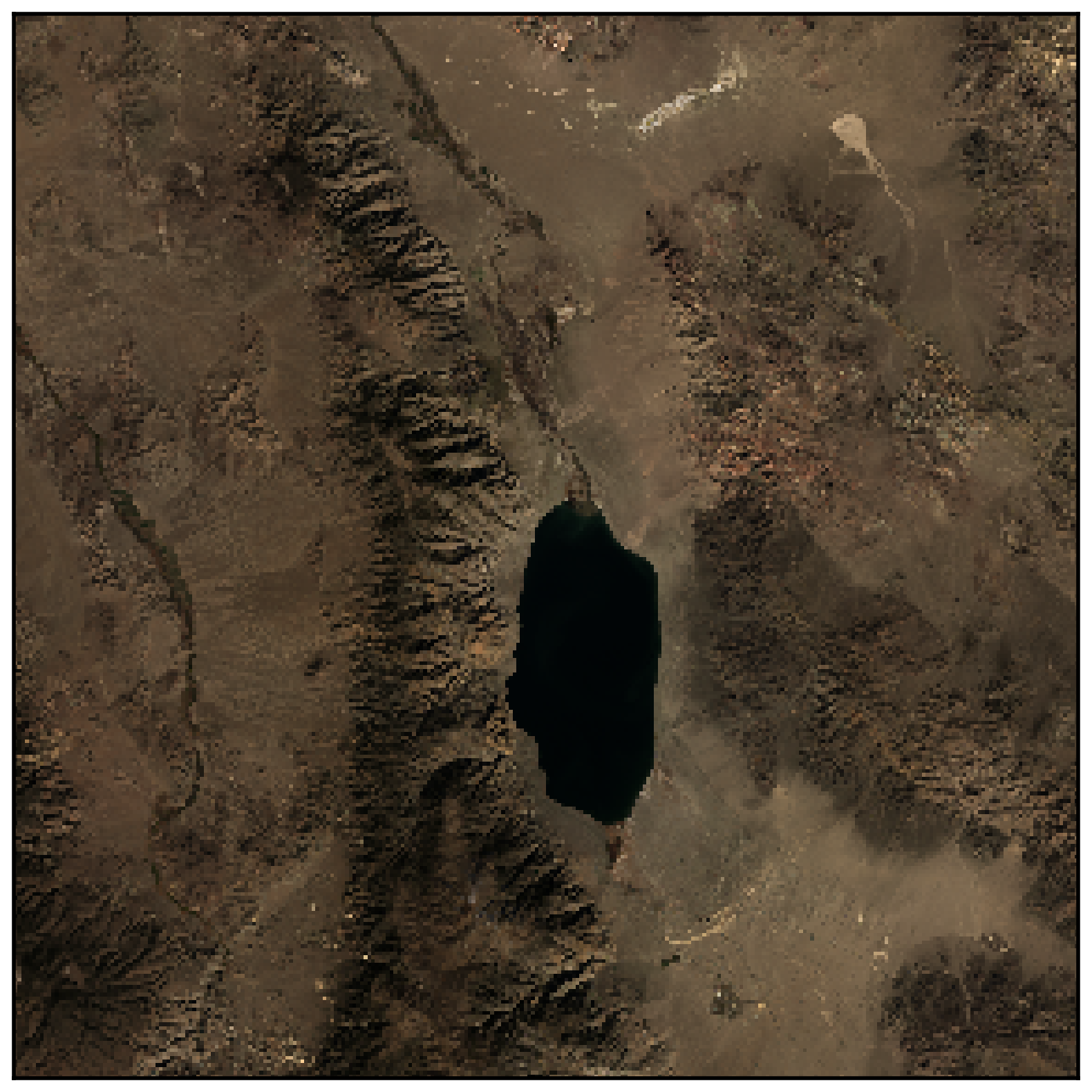

Landsat 5 color image

# Get the RGB data from landsat 5 dataset as a numpy array
rgb_data_5 = landsat_5_da.sel(band=[3,2,1]).values

# # Initialize
fig, ax = plt.subplots(figsize=(10,10))

# # Plot the RGB bands
ep.plot_rgb(rgb_data_5, rgb=(0, 1, 2), ax=ax);

Can we trim these to the same areas?

Yes, we can use xarray builtin selection functionality!

The Landsat 5 images is more zoomed in, so let’s trim to the Landsat 8 data to this range

Take advantage of the “coordinate” arrays provided by xarray:

landsat_5_da.x

<xarray.DataArray 'x' (x: 300)>
array([332400., 332550., 332700., ..., 376950., 377100., 377250.])
Coordinates:
  * x            (x) float64 3.324e+05 3.326e+05 ... 3.771e+05 3.772e+05
    spatial_ref  int64 0

xarray.DataArray

'x'

x: 300

3.324e+05 3.326e+05 3.327e+05 ... 3.77e+05 3.771e+05 3.772e+05

array([332400., 332550., 332700., ..., 376950., 377100., 377250.])

Coordinates: (2)
- x
  (x)
  float64
  3.324e+05 3.326e+05 ... 3.772e+05
```
array([332400., 332550., 332700., ..., 376950., 377100., 377250.])
```
- spatial_ref
  ()
  int64
  0
  crs_wkt :
  PROJCS["WGS 84 / UTM zone 11N",GEOGCS["WGS 84",DATUM["WGS_1984",SPHEROID["WGS 84",6378137,298.257223563,AUTHORITY["EPSG","7030"]],AUTHORITY["EPSG","6326"]],PRIMEM["Greenwich",0,AUTHORITY["EPSG","8901"]],UNIT["degree",0.0174532925199433,AUTHORITY["EPSG","9122"]],AUTHORITY["EPSG","4326"]],PROJECTION["Transverse_Mercator"],PARAMETER["latitude_of_origin",0],PARAMETER["central_meridian",-117],PARAMETER["scale_factor",0.9996],PARAMETER["false_easting",500000],PARAMETER["false_northing",0],UNIT["metre",1,AUTHORITY["EPSG","9001"]],AXIS["Easting",EAST],AXIS["Northing",NORTH],AUTHORITY["EPSG","32611"]]
  semi_major_axis :
  6378137.0
  semi_minor_axis :
  6356752.314245179
  inverse_flattening :
  298.257223563
  reference_ellipsoid_name :
  WGS 84
  longitude_of_prime_meridian :
  0.0
  prime_meridian_name :
  Greenwich
  geographic_crs_name :
  WGS 84
  horizontal_datum_name :
  World Geodetic System 1984
  projected_crs_name :
  WGS 84 / UTM zone 11N
  grid_mapping_name :
  transverse_mercator
  latitude_of_projection_origin :
  0.0
  longitude_of_central_meridian :
  -117.0
  false_easting :
  500000.0
  false_northing :
  0.0
  scale_factor_at_central_meridian :
  0.9996
  spatial_ref :
  PROJCS["WGS 84 / UTM zone 11N",GEOGCS["WGS 84",DATUM["WGS_1984",SPHEROID["WGS 84",6378137,298.257223563,AUTHORITY["EPSG","7030"]],AUTHORITY["EPSG","6326"]],PRIMEM["Greenwich",0,AUTHORITY["EPSG","8901"]],UNIT["degree",0.0174532925199433,AUTHORITY["EPSG","9122"]],AUTHORITY["EPSG","4326"]],PROJECTION["Transverse_Mercator"],PARAMETER["latitude_of_origin",0],PARAMETER["central_meridian",-117],PARAMETER["scale_factor",0.9996],PARAMETER["false_easting",500000],PARAMETER["false_northing",0],UNIT["metre",1,AUTHORITY["EPSG","9001"]],AXIS["Easting",EAST],AXIS["Northing",NORTH],AUTHORITY["EPSG","32611"]]
  GeoTransform :
  332325.0 150.0 0.0 4309275.0 0.0 -150.0
```
array(0)
```

Indexes: (1)

PandasIndex

PandasIndex(Float64Index([332400.0, 332550.0, 332700.0, 332850.0, 333000.0, 333150.0,
              333300.0, 333450.0, 333600.0, 333750.0,
              ...
              375900.0, 376050.0, 376200.0, 376350.0, 376500.0, 376650.0,
              376800.0, 376950.0, 377100.0, 377250.0],
             dtype='float64', name='x', length=300))

Attributes: (0)

landsat_5_da.y

<xarray.DataArray 'y' (y: 300)>
array([4309200., 4309050., 4308900., ..., 4264650., 4264500., 4264350.])
Coordinates:
  * y            (y) float64 4.309e+06 4.309e+06 ... 4.264e+06 4.264e+06
    spatial_ref  int64 0

xarray.DataArray

'y'

y: 300

4.309e+06 4.309e+06 4.309e+06 ... 4.265e+06 4.264e+06 4.264e+06

array([4309200., 4309050., 4308900., ..., 4264650., 4264500., 4264350.])

Coordinates: (2)
- y
  (y)
  float64
  4.309e+06 4.309e+06 ... 4.264e+06
```
array([4309200., 4309050., 4308900., ..., 4264650., 4264500., 4264350.])
```
- spatial_ref
  ()
  int64
  0
  crs_wkt :
  PROJCS["WGS 84 / UTM zone 11N",GEOGCS["WGS 84",DATUM["WGS_1984",SPHEROID["WGS 84",6378137,298.257223563,AUTHORITY["EPSG","7030"]],AUTHORITY["EPSG","6326"]],PRIMEM["Greenwich",0,AUTHORITY["EPSG","8901"]],UNIT["degree",0.0174532925199433,AUTHORITY["EPSG","9122"]],AUTHORITY["EPSG","4326"]],PROJECTION["Transverse_Mercator"],PARAMETER["latitude_of_origin",0],PARAMETER["central_meridian",-117],PARAMETER["scale_factor",0.9996],PARAMETER["false_easting",500000],PARAMETER["false_northing",0],UNIT["metre",1,AUTHORITY["EPSG","9001"]],AXIS["Easting",EAST],AXIS["Northing",NORTH],AUTHORITY["EPSG","32611"]]
  semi_major_axis :
  6378137.0
  semi_minor_axis :
  6356752.314245179
  inverse_flattening :
  298.257223563
  reference_ellipsoid_name :
  WGS 84
  longitude_of_prime_meridian :
  0.0
  prime_meridian_name :
  Greenwich
  geographic_crs_name :
  WGS 84
  horizontal_datum_name :
  World Geodetic System 1984
  projected_crs_name :
  WGS 84 / UTM zone 11N
  grid_mapping_name :
  transverse_mercator
  latitude_of_projection_origin :
  0.0
  longitude_of_central_meridian :
  -117.0
  false_easting :
  500000.0
  false_northing :
  0.0
  scale_factor_at_central_meridian :
  0.9996
  spatial_ref :
  PROJCS["WGS 84 / UTM zone 11N",GEOGCS["WGS 84",DATUM["WGS_1984",SPHEROID["WGS 84",6378137,298.257223563,AUTHORITY["EPSG","7030"]],AUTHORITY["EPSG","6326"]],PRIMEM["Greenwich",0,AUTHORITY["EPSG","8901"]],UNIT["degree",0.0174532925199433,AUTHORITY["EPSG","9122"]],AUTHORITY["EPSG","4326"]],PROJECTION["Transverse_Mercator"],PARAMETER["latitude_of_origin",0],PARAMETER["central_meridian",-117],PARAMETER["scale_factor",0.9996],PARAMETER["false_easting",500000],PARAMETER["false_northing",0],UNIT["metre",1,AUTHORITY["EPSG","9001"]],AXIS["Easting",EAST],AXIS["Northing",NORTH],AUTHORITY["EPSG","32611"]]
  GeoTransform :
  332325.0 150.0 0.0 4309275.0 0.0 -150.0
```
array(0)
```

Indexes: (1)

PandasIndex

PandasIndex(Float64Index([4309200.0, 4309050.0, 4308900.0, 4308750.0, 4308600.0, 4308450.0,
              4308300.0, 4308150.0, 4308000.0, 4307850.0,
              ...
              4265700.0, 4265550.0, 4265400.0, 4265250.0, 4265100.0, 4264950.0,
              4264800.0, 4264650.0, 4264500.0, 4264350.0],
             dtype='float64', name='y', length=300))

Attributes: (0)

Remember: These coordinates are in units of meters!

Let’s get the bounds of the Landsat 5 image:

# x bounds
xmin = landsat_5_da.x.min()
xmax = landsat_5_da.x.max()

# y bounds
ymin = landsat_5_da.y.min()
ymax = landsat_5_da.y.max()

Slicing with xarray

We can use Python’s built-in slice() function to slice the data’s coordinate arrays and select the subset of the data we want.

More info: http://xarray.pydata.org/en/stable/indexing.html

Slicing in Python

A slice object is used to specify how to slice a sequence.
You can specify where to start the slicing, and where to end. You can also specify the step, which allows you to e.g. slice only every other item.

Syntax: slice(start, end, step)

More info: https://www.w3schools.com/python/ref_func_slice.asp

An example

letters = ["a", "b", "c", "d", "e", "f", "g", "h"]

letters[0:5:2]

['a', 'c', 'e']

letters[slice(0, 5, 2)]

['a', 'c', 'e']

Back to xarray and the Landsat data…

We can use the .sel() function to slice our x and y coordinate arrays!

xmax

<xarray.DataArray 'x' ()>
array(377250.)
Coordinates:
    spatial_ref  int64 0

# slice the x and y coordinates
slice_x = slice(xmin, xmax)
slice_y = slice(ymax, ymin) # IMPORTANT: y coordinate array is in descending order

slice_x

slice(<xarray.DataArray 'x' ()>
array(332400.)
Coordinates:
    spatial_ref  int64 0, <xarray.DataArray 'x' ()>
array(377250.)
Coordinates:
    spatial_ref  int64 0, None)

# Use the .sel() to slice
landsat_8_trimmed = landsat_8_da.sel(x=slice_x, y=slice_y)

Important

The y coordinate is stored in descending order, so the slice should be ordered the same way (from ymax to ymin)

Let’s look at the trimmed data

landsat_8_trimmed.shape

(7, 214, 213)

landsat_8_da.shape

(7, 286, 286)

landsat_8_trimmed

Plot the trimmed Landsat 8 data:

# Get the trimmed landsat 8 RGB data as a numpy array
rgb_data_8 = landsat_8_trimmed.sel(band=[4,3,2]).values

# # Initialize
fig, ax = plt.subplots(figsize=(10,10))

# # Plot the RGB bands
ep.plot_rgb(rgb_data_8, rgb=(0, 1, 2), ax=ax);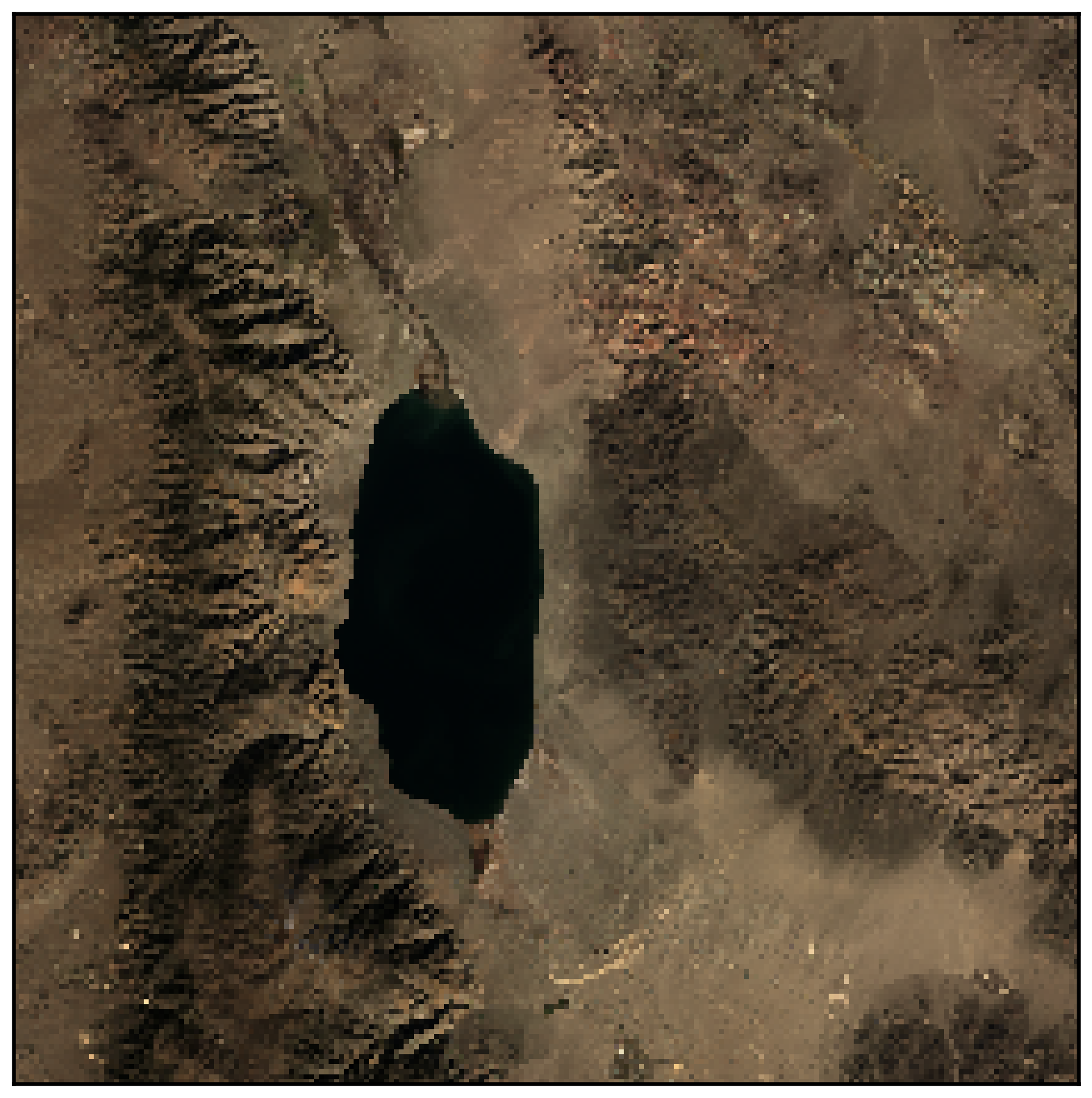

Plot the original Landsat 5 data:

# Select the RGB data as a numpy array
rgb_data_5 = landsat_5_da.sel(band=[3,2,1]).values

# Initialize the figure
fig, ax = plt.subplots(figsize=(10,10))

# Plot the RGB bands
ep.plot_rgb(rgb_data_5, rgb=(0, 1, 2), ax=ax);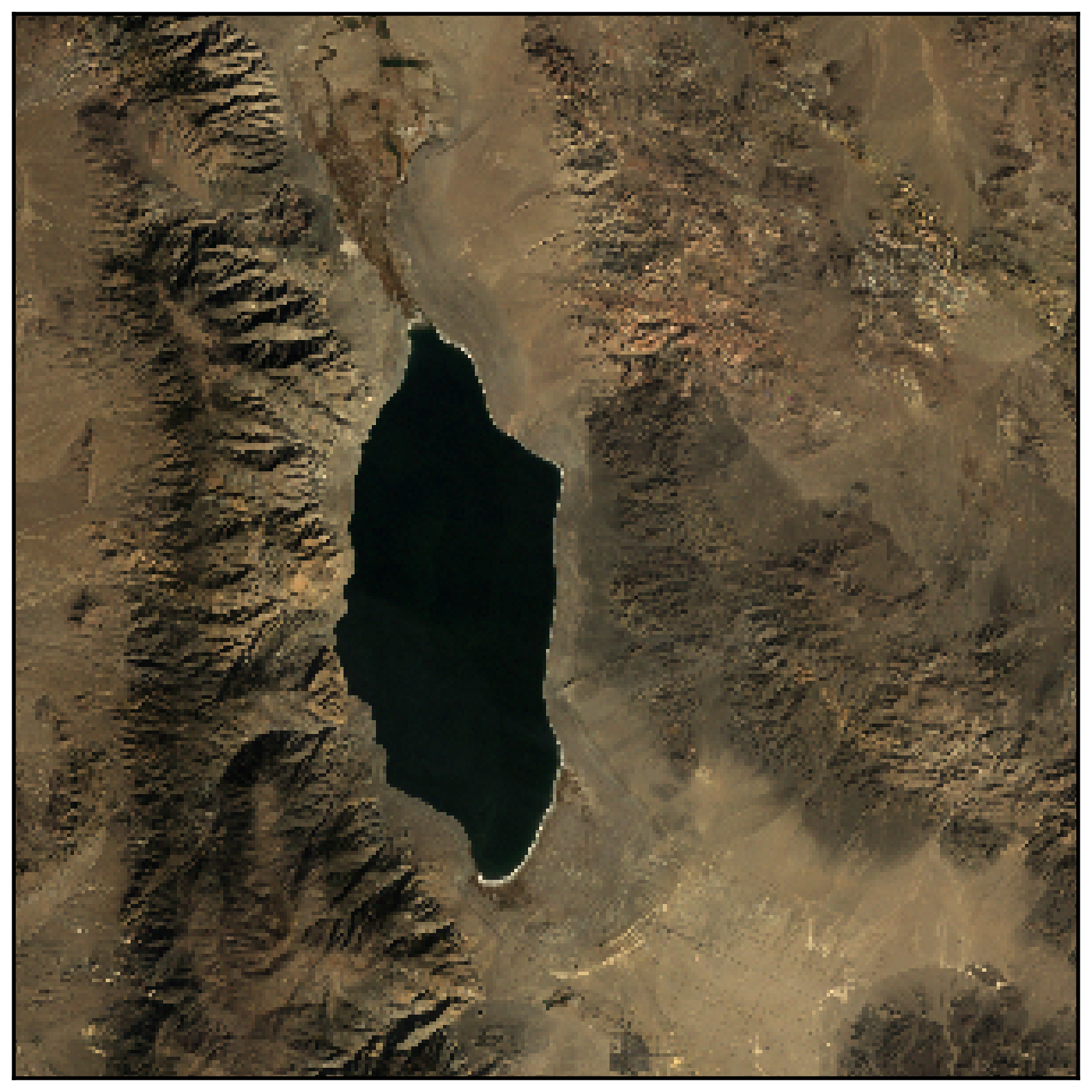

Some evidence of shrinkage…but can we do better?

Yes! We’ll use the change in the NDVI over time to detect change in lake volume

Calculate the NDVI for the Landsat 5 (1988) and Landsat 8 (2017) datasets

Remember

NDVI = (NIR - Red) / (NIR + Red)
You can once again use the .sel() function to select certain bands from the datasets

For Landsat 5: NIR = band 4 and Red = band 3

For Landsat 8: NIR = band 5 and Red = band 4

NDVI 1988

NIR_1988 = landsat_5_da.sel(band=4)
RED_1988 = landsat_5_da.sel(band=3)

NDVI_1988 = (NIR_1988 - RED_1988) / (NIR_1988 + RED_1988)

NDVI 2017

NIR_2017 = landsat_8_da.sel(band=5)
RED_2017 = landsat_8_da.sel(band=4)

NDVI_2017 = (NIR_2017 - RED_2017) / (NIR_2017 + RED_2017)

The difference between 2017 and 1988

Take the difference between the 2017 NDVI and the 1988 NDVI
Use the hvplot.image() function to show the difference
A diverging palette, like coolwarm, is particularly useful for this situation

diff = NDVI_2017 - NDVI_1988

diff.hvplot.image(
    x="x",
    y="y",
    frame_height=400,
    frame_width=400,
    cmap="coolwarm",
    clim=(-1, 1),
    geo=True,
    crs=32611,
)

/Users/nhand/mambaforge/envs/musa-550-fall-2023/lib/python3.10/site-packages/osgeo/osr.py:385: FutureWarning: Neither osr.UseExceptions() nor osr.DontUseExceptions() has been explicitly called. In GDAL 4.0, exceptions will be enabled by default.
  warnings.warn(

NDVI_1988.shape

(300, 300)

NDVI_2017.shape

(286, 286)

diff.shape

(42, 43)

What’s going on here? Why so pixelated?

Two issues: - Different x/y bounds - Different resolutions

# Different x/y ranges!
print(NDVI_1988.x[0].values)
print(NDVI_2017.x[0].values)

332400.0
318300.0

# Different resolutions
print((NDVI_1988.x[1] - NDVI_1988.x[0]).values)
print((NDVI_2017.x[1] - NDVI_2017.x[0]).values)

150.0
210.0

Use xarray to put the data on the same grid

First, calculate a bounding box around the center of the data

# The center lat/lng values in EPSG = 4326
# I got these points from google maps 
x0 = -118.7081
y0 = 38.6942

Let’s convert these coordinates to the sames CRS as the Landsat data

We can also use geopandas:

pt = pd.DataFrame({"lng": [x0], "lat": [y0]})

gpt = gpd.GeoDataFrame(
    pt, geometry=gpd.points_from_xy(pt["lng"], pt["lat"]), crs="EPSG:4326"
)

gpt

	lng	lat	geometry
0	-118.7081	38.6942	POINT (-118.70810 38.69420)

Convert to the Landsat CRS. Remember: we are converting from EPSG=4326 to EPSG=32611

pt_32611 = gpt.to_crs(epsg=32611)

Let’s add a circle with radius 15 km around the midpoint

pt_32611_buffer = pt_32611.copy()
pt_32611_buffer.geometry = pt_32611.geometry.buffer(15e3)  # Add a 15 km radius buffer

Did this work?

Use the builting geoviews imagery to confirm..

EsriImagery * pt_32611_buffer.hvplot(alpha=0.4, geo=True, crs=32611)

Now, let’s set up the grid

res = 200 # 200 meter resolution
x = np.arange(xmin, xmax, res)
y = np.arange(ymin, ymax, res)

len(x)

len(y)

Do the re-gridding

This does a linear interpolation of the data using the nearest pixels.

NDVI_2017_regridded = NDVI_2017.interp(x=x, y=y)
NDVI_1988_regridded = NDVI_1988.interp(x=x, y=y)

Plot the re-gridded data side-by-side

img1988 = NDVI_1988_regridded.hvplot.image(
    x="x",
    y="y",
    crs=32611,
    geo=True,
    frame_height=300,
    frame_width=300,
    clim=(-3, 1),
    cmap="fire",
    title="1988"
)


img2017 = NDVI_2017_regridded.hvplot.image(
    x="x",
    y="y",
    crs=32611,
    geo=True,
    frame_height=300,
    frame_width=300,
    clim=(-3, 1),
    cmap="fire",
    title="2017"
)

img1988 + img2017

Now that the images are lined up, the change in lake volume is clearly apparent

diff_regridded = NDVI_2017_regridded - NDVI_1988_regridded
diff_regridded

diff_regridded.hvplot.image(
    x="x",
    y="y",
    crs=32611,
    geo=True,
    frame_height=400,
    frame_width=400,
    cmap="coolwarm",
    clim=(-1, 1),
)

Takeaway:

The red areas (more vegetation in 2017) show clear loss of lake volume

One more thing: downsampling hi-res data

Given hi-resolution data, we can downsample to a lower resolution with the familiar groupby / mean framework from pandas

Let’s try a resolution of 1000 meters instead of 200 meters

# Define a low-resolution grid
res_1000 = 1000
x_1000 = np.arange(xmin, xmax, res_1000)
y_1000 = np.arange(ymin, ymax, res_1000)

# Groupby new bins and take the mean of all pixels falling into a group
# First: groupby low-resolution x bins and take mean
# Then: groupby low-resolution y bins and take mean
diff_res_1000 = (
    diff_regridded.groupby_bins("x", x_1000, labels=x_1000[:-1])
    .mean(dim="x")
    .groupby_bins("y", y_1000, labels=y_1000[:-1])
    .mean(dim="y")
    .rename(x_bins="x", y_bins="y")
)
diff_res_1000

Now let’s plot the low-resolution version of the difference

diff_res_1000.hvplot.image(
    x="x",
    y="y",
    crs=32611,
    geo=True,
    frame_width=500,
    frame_height=400,
    cmap="coolwarm",
    clim=(-1, 1),
)

Example 2: urban heat islands

We’ll reproduce an analysis by Urban Spatial on urban heat islands in Philadelphia using Python.
The analysis uses Landsat 8 data (2017)
See: http://urbanspatialanalysis.com/urban-heat-islands-street-trees-in-philadelphia/

First load some metadata for Landsat 8

band_info = pd.DataFrame([
        (1,  "Aerosol", " 0.43 - 0.45",    0.440,  "30",         "Coastal aerosol"),
        (2,  "Blue",    " 0.45 - 0.51",    0.480,  "30",         "Blue"),
        (3,  "Green",   " 0.53 - 0.59",    0.560,  "30",         "Green"),
        (4,  "Red",     " 0.64 - 0.67",    0.655,  "30",         "Red"),
        (5,  "NIR",     " 0.85 - 0.88",    0.865,  "30",         "Near Infrared (NIR)"),
        (6,  "SWIR1",   " 1.57 - 1.65",    1.610,  "30",         "Shortwave Infrared (SWIR) 1"),
        (7,  "SWIR2",   " 2.11 - 2.29",    2.200,  "30",         "Shortwave Infrared (SWIR) 2"),
        (8,  "Panc",    " 0.50 - 0.68",    0.590,  "15",         "Panchromatic"),
        (9,  "Cirrus",  " 1.36 - 1.38",    1.370,  "30",         "Cirrus"),
        (10, "TIRS1",   "10.60 - 11.19",   10.895, "100 * (30)", "Thermal Infrared (TIRS) 1"),
        (11, "TIRS2",   "11.50 - 12.51",   12.005, "100 * (30)", "Thermal Infrared (TIRS) 2")],
    columns=['Band', 'Name', 'Wavelength Range (µm)', 'Nominal Wavelength (µm)', 'Resolution (m)', 'Description']).set_index(["Band"])
band_info

	Name	Wavelength Range (µm)	Nominal Wavelength (µm)	Resolution (m)	Description
Band
1	Aerosol	0.43 - 0.45	0.440	30	Coastal aerosol
2	Blue	0.45 - 0.51	0.480	30	Blue
3	Green	0.53 - 0.59	0.560	30	Green
4	Red	0.64 - 0.67	0.655	30	Red
5	NIR	0.85 - 0.88	0.865	30	Near Infrared (NIR)
6	SWIR1	1.57 - 1.65	1.610	30	Shortwave Infrared (SWIR) 1
7	SWIR2	2.11 - 2.29	2.200	30	Shortwave Infrared (SWIR) 2
8	Panc	0.50 - 0.68	0.590	15	Panchromatic
9	Cirrus	1.36 - 1.38	1.370	30	Cirrus
10	TIRS1	10.60 - 11.19	10.895	100 * (30)	Thermal Infrared (TIRS) 1
11	TIRS2	11.50 - 12.51	12.005	100 * (30)	Thermal Infrared (TIRS) 2

Landsat data on Google Cloud Storage

We’ll be downloading publicly available Landsat data from Google Cloud Storage

See: https://cloud.google.com/storage/docs/public-datasets/landsat

The relevant information is stored in our intake catalog:

From our catalog.yml file:

google_landsat_band:
    description: Landsat bands from Google Cloud Storage
    driver: rasterio
    parameters:
      path:
        description: landsat path
        type: int
      row:
        description: landsat row
        type: int
      product_id:
        description: landsat file id
        type: str
      band:
        description: band
        type: int
    args:
      urlpath: https://storage.googleapis.com/gcp-public-data-landsat/LC08/01/{{ '%03d' % path }}/{{ '%03d' % row }}/{{ product_id }}/{{ product_id }}_B{{ band }}.TIF
      chunks:
        band: 1
        x: 256
        y: 256

From the “urlpath” above, you can see we need “path”, “row”, and “product_id” variables to properly identify a Landsat image:

The path and row corresponding to the area over Philadelphia has already been selected using the Earth Explorer. This tool was also used to find the id of the particular date of interest using the same tool.

# Necessary variables
path = 14
row = 32
product_id = 'LC08_L1TP_014032_20160727_20170222_01_T1'

An alternative: Google Earth Engine (GEE)

A public data archive of satellite imagery going back more than 40 years.
A Python API exists for pulling data — good resource if you’d like to work with a large amount of raster data

We won’t cover the specifics in the course, but geemap is a fantastic library for interacting with GEE.

References

Google Earth Engine (GEE):
geemap package:

Google Cloud Storage: Use a utility function to query the API and request a specific band

This will return a specific Landsat band as a dask array.

from random import random
from time import sleep


def get_band_with_exponential_backoff(path, row, product_id, band, maximum_backoff=32):
    """
    Google Cloud Storage recommends using exponential backoff 
    when accessing the API. 
    
    https://cloud.google.com/storage/docs/exponential-backoff
    """
    n = backoff = 0
    while backoff < maximum_backoff:
        try:
            return cat.google_landsat_band(
                path=path, row=row, product_id=product_id, band=band
            ).to_dask()
        except:
            backoff = min(2 ** n + random(), maximum_backoff)
            sleep(backoff)
            n += 1

Load all of the bands and combine them into a single xarray DataArray

Loop over each band, load that band using the above function, and then concatenate the results together..

bands = [1, 2, 3, 4, 5, 6, 7, 9, 10, 11]

datasets = []
for band in bands:
    da = get_band_with_exponential_backoff(
        path=path, row=row, product_id=product_id, band=band
    )
    da = da.assign_coords(band=[band])
    datasets.append(da)

ds = xr.concat(datasets, "band", compat="identical")

ds

<xarray.DataArray (band: 10, y: 7871, x: 7741)>
dask.array<concatenate, shape=(10, 7871, 7741), dtype=uint16, chunksize=(1, 256, 256), chunktype=numpy.ndarray>
Coordinates:
  * band         (band) int64 1 2 3 4 5 6 7 9 10 11
  * x            (x) float64 3.954e+05 3.954e+05 ... 6.276e+05 6.276e+05
  * y            (y) float64 4.582e+06 4.582e+06 ... 4.346e+06 4.346e+06
    spatial_ref  int64 0
Attributes:
    AREA_OR_POINT:  Point
    scale_factor:   1.0
    add_offset:     0.0

Important

CRS for Landsat data is EPSG=32618

Also grab the metadata from Google Cloud Storage

There is an associated metadata file stored on Google Cloud Storage
The below function will parse that metadata file for a specific path, row, and product ID
The specifics of this are not overly important for our purposes

def load_google_landsat_metadata(path, row, product_id):
    """
    Load Landsat metadata for path, row, product_id from Google Cloud Storage
    """

    def parse_type(x):
        try:
            return eval(x)
        except:
            return x

    baseurl = "https://storage.googleapis.com/gcp-public-data-landsat/LC08/01"
    suffix = f"{path:03d}/{row:03d}/{product_id}/{product_id}_MTL.txt"

    df = intake.open_csv(
        urlpath=f"{baseurl}/{suffix}",
        csv_kwargs={
            "sep": "=",
            "header": None,
            "names": ["index", "value"],
            "skiprows": 2,
            "converters": {"index": (lambda x: x.strip()), "value": parse_type},
        },
    ).read()
    metadata = df.set_index("index")["value"]
    return metadata

metadata = load_google_landsat_metadata(path, row, product_id)
metadata.head()

index
ORIGIN                Image courtesy of the U.S. Geological Survey
REQUEST_ID                                     0501702206266_00020
LANDSAT_SCENE_ID                             LC80140322016209LGN01
LANDSAT_PRODUCT_ID        LC08_L1TP_014032_20160727_20170222_01_T1
COLLECTION_NUMBER                                               01
Name: value, dtype: object

Exercise: Let’s trim our data to the Philadelphia limits

The Landsat image covers an area much wider than the Philadelphia limits
We’ll load the city limits from Open Data Philly
Use the slice() function discussed last example!

1. Load the city limits

From OpenDataPhilly, the city limits for Philadelphia are available at: http://data.phl.opendata.arcgis.com/datasets/405ec3da942d4e20869d4e1449a2be48_0.geojson
Be sure to convert to the same CRS as the Landsat data!

# Load the GeoJSON from the URL
url = "http://data.phl.opendata.arcgis.com/datasets/405ec3da942d4e20869d4e1449a2be48_0.geojson"
city_limits = gpd.read_file(url)

# Convert to the right CRS for this data
city_limits = city_limits.to_crs(epsg=32618)

2. Use the xmin/xmax and ymin/ymax of the city limits to trim the Landsat DataArray

Use the built-in slice functionality of xarray
Remember, the y coordinates are in descending order, so you’ll slice will need to be in descending order as well

city_limits.total_bounds?

Type:        property
String form: <property object at 0x13fa2dc60>
Docstring:  
Returns a tuple containing ``minx``, ``miny``, ``maxx``, ``maxy``
values for the bounds of the series as a whole.
See ``GeoSeries.bounds`` for the bounds of the geometries contained in
the series.
Examples
--------
>>> from shapely.geometry import Point, Polygon, LineString
>>> d = {'geometry': [Point(3, -1), Polygon([(0, 0), (1, 1), (1, 0)]),
... LineString([(0, 1), (1, 2)])]}
>>> gdf = geopandas.GeoDataFrame(d, crs="EPSG:4326")
>>> gdf.total_bounds
array([ 0., -1.,  3.,  2.])

# Get x/y range of city limits from "total_bounds"
xmin, ymin, xmax, ymax = city_limits.total_bounds

# Slice our xarray data
subset = ds.sel(
                x=slice(xmin, xmax), 
                y=slice(ymax, ymin)
               ) # NOTE: y coordinate system is in descending order!

Step 3: Call the compute() function on your sliced data

Originally, the Landsat data was stored as dask arrays
This should now only load the data into memory that covers Philadelphia

This should take about a minute or so, depending on the speed of your laptop.

subset = subset.compute()

subset

# Original data was about 8000 x 8000 in size
ds.shape

(10, 7871, 7741)

# Sliced data is only about 1000 x 1000 in size!
subset.shape

(10, 1000, 924)

Last two lectures!

The decline of the world’s saline lakes

The Aral Sea in Kazakhstan

2000

2018

Lake Urmia in Iran

1998

2011

Today: Walker Lake

1988

2017

Let’s analyze this in Python!

First, let’s use intake to load the data

Intake let’s you define “default” plots for a dataset

What’s happening under the hood?

We can do the same for the Landsat 8 data

We can use dask to read the data

Use “.values” to convert to a numpy array

Evidence of shrinkage?

First: Let’s plot RGB images of the two datasets

Important notes

Landsat 8 color image

Landsat 5 color image

Can we trim these to the same areas?

Slicing with xarray

Slicing in Python

An example

Back to xarray and the Landsat data…

Let’s look at the trimmed data

Calculate the NDVI for the Landsat 5 (1988) and Landsat 8 (2017) datasets

NDVI 1988

NDVI 2017

The difference between 2017 and 1988

What’s going on here? Why so pixelated?

Use xarray to put the data on the same grid

First, calculate a bounding box around the center of the data

Did this work?

Now, let’s set up the grid

Do the re-gridding

Plot the re-gridded data side-by-side

Takeaway:

One more thing: downsampling hi-res data

Now let’s plot the low-resolution version of the difference

Example 2: urban heat islands

First load some metadata for Landsat 8

Landsat data on Google Cloud Storage

An alternative: Google Earth Engine (GEE)

References

Google Cloud Storage: Use a utility function to query the API and request a specific band

Load all of the bands and combine them into a single xarray DataArray

Also grab the metadata from Google Cloud Storage

Exercise: Let’s trim our data to the Philadelphia limits

1. Load the city limits

2. Use the xmin/xmax and ymin/ymax of the city limits to trim the Landsat DataArray

Step 3: Call the compute() function on your sliced data

To be continued!