Lecture 13A: Predictive modeling with scikit-learn, continued

from matplotlib import pyplot as plt
import numpy as np
import pandas as pd
import geopandas as gpd
import requests
import hvplot.pandas

np.random.seed(42)

pd.options.display.max_columns = 999

• Nov 29, 2023
• Section 401

Predictive modeling, continued

Focus: much more hands-on experience with featuring engineering and adding spatial based features

• Part 1: Housing price modeling
• Part 2: Predicting bikeshare demand in Philadelphia

Recap

• An introduction to supervised learning and regression with scikit learn
• Key concepts:
  • Linear regression
  • Ridge regression with regularization
  • Test/train split and k-fold cross validation
  • Feature engineering
    • Scaling input features
    • Adding polynomial features
    • One-hot encoding + categorical variables
  • Decision trees and random forests

Today: modeling housing prices in Philadelphia

First, let’s setup all of the imports we’ll need from scikit learn:

# Models
from sklearn.linear_model import LinearRegression
from sklearn.ensemble import RandomForestRegressor

# Model selection
from sklearn.model_selection import train_test_split, cross_val_score, GridSearchCV

# Pipelines
from sklearn.pipeline import make_pipeline

# Preprocessing
from sklearn.preprocessing import StandardScaler, PolynomialFeatures

Review: Predicting housing prices in Philadelphia

Load data from the Office of Property Assessment

Let’s download data for single-family properties in Philadelphia that had their last sale during 2022.

Sources: - OpenDataPhilly - Metadata

Download the raw sales data:

# the CARTO API url
carto_url = "https://phl.carto.com/api/v2/sql"

# Only pull 2022 sales for single family residential properties
where = "sale_date >= '2022-01-01' and sale_date <= '2022-12-31'"
where = where + " and category_code_description IN ('SINGLE FAMILY', 'Single Family')"

# Create the query
query = f"SELECT * FROM opa_properties_public WHERE {where}"

# Make the request
params = {"q": query, "format": "geojson"}
response = requests.get(carto_url, params=params)

Convert to a GeoDataFrame:

# Make the GeoDataFrame
salesRaw = gpd.GeoDataFrame.from_features(response.json(), crs="EPSG:4326")

# Optional: put it a reproducible order for test/training splits later
salesRaw = salesRaw.sort_values("parcel_number")

salesRaw.head()

	geometry	cartodb_id	assessment_date	basements	beginning_point	book_and_page	building_code	building_code_description	category_code	category_code_description	census_tract	central_air	cross_reference	date_exterior_condition	depth	exempt_building	exempt_land	exterior_condition	fireplaces	frontage	fuel	garage_spaces	garage_type	general_construction	geographic_ward	homestead_exemption	house_extension	house_number	interior_condition	location	mailing_address_1	mailing_address_2	mailing_care_of	mailing_city_state	mailing_street	mailing_zip	market_value	market_value_date	number_of_bathrooms	number_of_bedrooms	number_of_rooms	number_stories	off_street_open	other_building	owner_1	owner_2	parcel_number	parcel_shape	quality_grade	recording_date	registry_number	sale_date	sale_price	separate_utilities	sewer	site_type	state_code	street_code	street_designation	street_direction	street_name	suffix	taxable_building	taxable_land	topography	total_area	total_livable_area	type_heater	unfinished	unit	utility	view_type	year_built	year_built_estimate	zip_code	zoning	pin	building_code_new	building_code_description_new	objectid
966	POINT (-75.14860 39.93145)	16819	2022-05-24T00:00:00Z	0	36'6" E OF AMERICAN	54131081	R30	ROW B/GAR 2 STY MASONRY	1	SINGLE FAMILY	27	Y	None	None	90.0	0.0	0.0	4	0.0	18.0	None	1.0	None	A	1	0	None	224	4	224 WHARTON ST	SIMPLIFILE LC E-RECORDING	None	None	PHILADELPHIA PA	224 WHARTON ST	19147-5336	327600	None	2.0	3.0	NaN	3.0	711.0	None	DEVER CATHERINE JOAN	None	011001670	E	C	2022-12-14T00:00:00Z	9S17 307	2022-12-05T00:00:00Z	450000	None	None	None	PA	82740	ST	None	WHARTON	None	262080.0	65520.0	F	1625.0	1785.0	A	None	None	None	I	1960	Y	19147	RSA5	1001563093	26	ROW RIVER ROW	397028047
12147	POINT (-75.14817 39.93101)	31147	2022-05-24T00:00:00Z	A	50' W SIDE OF 2ND ST	54063610	O50	ROW 3 STY MASONRY	1	SINGLE FAMILY	27	Y	None	None	36.0	80000.0	0.0	3	0.0	34.0	A	0.0	None	A	1	80000	None	205	3	205 EARP ST	SIMPLIFILE LC E-RECORDING	None	None	PHILADELPHIA PA	205 EARP ST	19147-6035	434400	None	3.0	4.0	NaN	3.0	467.0	None	MORAN KELLY	TRENTALANGE SILVIO	011004720	E	C+	2022-06-30T00:00:00Z	009S170369	2022-06-24T00:00:00Z	670000	A	None	None	PA	30420	ST	None	EARP	None	267520.0	86880.0	F	1224.0	2244.0	A	None	None	None	I	2009	None	19147	RSA5	1001190209	22	ROW TYPICAL	397041168
7323	POINT (-75.14781 39.93010)	25174	2022-05-24T00:00:00Z	A	33.333 S OF REED	54085418	P51	ROW W/GAR 3 STY MAS+OTHER	1	SINGLE FAMILY	27	Y	None	None	84.0	574320.0	0.0	1	0.0	17.0	A	1.0	None	C	1	0	None	136	1	136 REED ST	SIMPLIFILE LC E-RECORDING	None	None	PHILADELPHIA PA	136 REED ST	19147-6117	717900	None	0.0	3.0	NaN	2.0	296.0	None	DOLIN CARLY P	DOLIN RYAN N	011011410	E	C+	2022-08-16T00:00:00Z	010S110342	2022-08-09T00:00:00Z	790000	None	Y	None	PA	67780	ST	None	REED	None	0.0	143580.0	F	1400.0	2514.0	A	None	None	None	I	2014	None	19147	ICMX	1001442221	25	ROW MODERN	397036560
2198	POINT (-75.14887 39.93026)	18788	2022-05-24T00:00:00Z	D	68 FT W PHILIP ST	54127951	O50	ROW 3 STY MASONRY	1	SINGLE FAMILY	27	Y	None	None	60.0	180200.0	0.0	4	0.0	14.0	None	0.0	None	A	1	0	None	220	4	220 REED ST	OLKOWSKI KEITH	None	None	PHILADELPHIA PA	243 GREENWICH STREET	19147	293000	None	2.0	3.0	NaN	3.0	193.0	None	OLKOWSKI KEITH	RACHUBINSKI MICHAEL	011012200	E	C	2022-12-06T00:00:00Z	010S110109	2022-12-02T00:00:00Z	195000	None	None	None	PA	67780	ST	None	REED	None	54200.0	58600.0	F	840.0	1358.0	H	None	None	None	I	1920	Y	19147	RSA5	1001442236	22	ROW TYPICAL	397028550
16292	POINT (-75.14881 39.93012)	31111	2022-05-24T00:00:00Z	D	42 FT W PHILIP	54063384	O30	ROW 2 STY MASONRY	1	SINGLE FAMILY	27	Y	None	None	39.0	0.0	0.0	3	0.0	14.0	None	0.0	None	A	1	0	None	207	3	207 GERRITT ST	SIMPLIFILE LC E-RECORDING	None	None	PHILADELPHIA PA	207 GERRITT ST	19147-6012	255500	None	2.0	2.0	NaN	2.0	141.0	None	NETTER DANIEL ANTHONY	NETTER SARAH ANNE	011014000	E	C	2022-06-29T00:00:00Z	010S110172	2022-06-27T00:00:00Z	331000	None	None	None	PA	36680	ST	None	GERRITT	None	204400.0	51100.0	F	546.0	868.0	H	None	None	None	I	1920	Y	19147	RSA5	1001238775	22	ROW TYPICAL	397041384

len(salesRaw)

24456

Get the feature sales data we will work with:

# The feature columns we want to use
cols = [
    "sale_price",
    "total_livable_area",
    "total_area",
    "garage_spaces",
    "fireplaces",
    "number_of_bathrooms",
    "number_of_bedrooms",
    "number_stories",
    "exterior_condition",
    "zip_code",
]

# Trim to these columns and remove NaNs
sales = salesRaw[cols + ["geometry"]].dropna()

# Trim zip code to only the first five digits
sales["zip_code"] = sales["zip_code"].astype(str).str.slice(0, 5)

# Trim very low and very high sales
valid = (sales['sale_price'] > 3000) & (sales['sale_price'] < 1e6)
sales = sales.loc[valid]

len(sales)

17675

Let’s focus on numerical features only first

Split the data into a training and test set:

# Split the data 70/30
train_set, test_set = train_test_split(sales, test_size=0.3, random_state=42)

Get the predictive variable: log of sale price:

# the target labels: log of sale price
y_train = np.log(train_set["sale_price"])
y_test = np.log(test_set["sale_price"])

Get the features (numerical only first):

# The features
feature_cols = [
    "total_livable_area",
    "total_area",
    "garage_spaces",
    "fireplaces",
    "number_of_bathrooms",
    "number_of_bedrooms",
    "number_stories",
]
X_train = train_set[feature_cols].values
X_test = test_set[feature_cols].values

Run a linear regression model as a baseline:

# Make a linear model pipeline
linear_pipeline = make_pipeline(StandardScaler(), LinearRegression())

# Fit on the training data
linear_pipeline.fit(X_train, y_train)

# What's the test score?
linear_pipeline.score(X_test, y_test)

0.18465378246963382

Run cross-validation on a random forest model:

# Make a random forest pipeline
forest_pipeline = make_pipeline(
    StandardScaler(), RandomForestRegressor(n_estimators=100, random_state=42)
)

# Run the 10-fold cross validation
scores = cross_val_score(
    forest_pipeline,
    X_train,
    y_train,
    cv=10,
)

# Report
print("R^2 scores = ", scores)
print("Scores mean = ", scores.mean())
print("Score std dev = ", scores.std())

R^2 scores =  [0.32549221 0.36405574 0.31498968 0.29773715 0.32731989 0.26301082
 0.3237037  0.32231956 0.28549553 0.35235816]
Scores mean =  0.3176482454802408
Score std dev =  0.028274645959991906

# Fit on the training data
forest_pipeline.fit(X_train, y_train)

# What's the test score?
forest_pipeline.score(X_test, y_test)

0.32708994151649196

Which variables were most important?

# Extract the regressor from the pipeline
forest_model = forest_pipeline["randomforestregressor"]

# Create the data frame of importances
importance = pd.DataFrame(
    {"Feature": feature_cols, "Importance": forest_model.feature_importances_}
).sort_values("Importance")


importance.hvplot.barh(x="Feature", y="Importance")

How to handle categorical data?

We can use a technique called one-hot encoding

Steps: - Create a new column for each category - Represent each category as a vector of 1s and 0s

One-hot encoding in scikit learn

• The OneHotEncoder object is a preprocessor that will perform the vectorization step
• The ColumnTransformer object will help us apply different transformers to numerical and categorical columns

from sklearn.compose import ColumnTransformer
from sklearn.preprocessing import OneHotEncoder

Let’s try out the example data of colors:

# Example data of colors
colors = np.array(["red", "green", "blue", "red"])
colors = colors[:, np.newaxis]

colors.shape

(4, 1)

colors

array([['red'],
       ['green'],
       ['blue'],
       ['red']], dtype='<U5')

# Initialize the OHE transformer
ohe = OneHotEncoder()

# Fit the transformer and then transform the colors 
ohe.fit_transform(colors).toarray()

array([[0., 0., 1.],
       [0., 1., 0.],
       [1., 0., 0.],
       [0., 0., 1.]])

# The corresponding category for each column
ohe.categories_

[array(['blue', 'green', 'red'], dtype='<U5')]

Let’s apply separate transformers for our numerical and categorical columns:

# Numerical columns
num_cols = [
    "total_livable_area",
    "total_area",
    "garage_spaces",
    "fireplaces",
    "number_of_bathrooms",
    "number_of_bedrooms",
    "number_stories",
]

# Categorical columns
cat_cols = ["exterior_condition", "zip_code"]

# Set up the column transformer with two transformers
# ----> Scale the numerical columns
# ----> One-hot encode the categorical columns

transformer = ColumnTransformer(
    transformers=[
        ("num", StandardScaler(), num_cols),
        ("cat", OneHotEncoder(handle_unknown="ignore"), cat_cols),
    ]
)

Note: the handle_unknown='ignore' parameter ensures that if categories show up in our training set, but not our test set, no error will be raised.

Initialize the pipeline object, using the column transformer and the random forest regressor

# Initialize the pipeline
# NOTE: only use 10 estimators here so it will run in a reasonable time
pipe = make_pipeline(
    transformer, RandomForestRegressor(n_estimators=10, 
                                       random_state=42)
)

Now, let’s fit the model.

Important!

• You must pass in the full training set and test set DataFrames: train_set and test_set
• No need to create the X_train and X_test numpy arrays.
• We told scikit learn which column strings to extract in the ColumnTransformer, so it needs the DataFrame with named columns.

# Fit the training set
pipe.fit(train_set, y_train);

# What's the test score?
pipe.score(test_set, y_test)

0.5124718138334259

Substantial improvement on test set when including ZIP codes

R-squared of ~0.30 improved to R-squared of ~0.53!

Takeaway: neighborhood based effects play a crucial role in determining housing prices.

Side Note: to fully validate the model we should run k-fold cross validation and optimize hyperparameters of the model as well…

But how crucial? Let’s plot the importances

But first, we need to know the column names! The one-hot encoder created a column for each category type…

# The column transformer...
transformer

ColumnTransformer(transformers=[('num', StandardScaler(),
                                 ['total_livable_area', 'total_area',
                                  'garage_spaces', 'fireplaces',
                                  'number_of_bathrooms', 'number_of_bedrooms',
                                  'number_stories']),
                                ('cat', OneHotEncoder(handle_unknown='ignore'),
                                 ['exterior_condition', 'zip_code'])])

In a Jupyter environment, please rerun this cell to show the HTML representation or trust the notebook.
On GitHub, the HTML representation is unable to render, please try loading this page with nbviewer.org.

# The steps in the column transformer
transformer.named_transformers_

{'num': StandardScaler(),
 'cat': OneHotEncoder(handle_unknown='ignore'),
 'remainder': 'drop'}

# The one-hot step
ohe = transformer.named_transformers_['cat']

ohe

OneHotEncoder(handle_unknown='ignore')

In a Jupyter environment, please rerun this cell to show the HTML representation or trust the notebook.
On GitHub, the HTML representation is unable to render, please try loading this page with nbviewer.org.

# One column for each category type!
ohe_cols = ohe.get_feature_names_out()

ohe_cols

array(['exterior_condition_0', 'exterior_condition_1',
       'exterior_condition_2', 'exterior_condition_3',
       'exterior_condition_4', 'exterior_condition_5',
       'exterior_condition_6', 'exterior_condition_7', 'zip_code_19102',
       'zip_code_19103', 'zip_code_19104', 'zip_code_19106',
       'zip_code_19107', 'zip_code_19111', 'zip_code_19114',
       'zip_code_19115', 'zip_code_19116', 'zip_code_19118',
       'zip_code_19119', 'zip_code_19120', 'zip_code_19121',
       'zip_code_19122', 'zip_code_19123', 'zip_code_19124',
       'zip_code_19125', 'zip_code_19126', 'zip_code_19127',
       'zip_code_19128', 'zip_code_19129', 'zip_code_19130',
       'zip_code_19131', 'zip_code_19132', 'zip_code_19133',
       'zip_code_19134', 'zip_code_19135', 'zip_code_19136',
       'zip_code_19137', 'zip_code_19138', 'zip_code_19139',
       'zip_code_19140', 'zip_code_19141', 'zip_code_19142',
       'zip_code_19143', 'zip_code_19144', 'zip_code_19145',
       'zip_code_19146', 'zip_code_19147', 'zip_code_19148',
       'zip_code_19149', 'zip_code_19150', 'zip_code_19151',
       'zip_code_19152', 'zip_code_19153', 'zip_code_19154'], dtype=object)

# Full list of columns is numerical + one-hot 
features = num_cols + list(ohe_cols)

features

['total_livable_area',
 'total_area',
 'garage_spaces',
 'fireplaces',
 'number_of_bathrooms',
 'number_of_bedrooms',
 'number_stories',
 'exterior_condition_0',
 'exterior_condition_1',
 'exterior_condition_2',
 'exterior_condition_3',
 'exterior_condition_4',
 'exterior_condition_5',
 'exterior_condition_6',
 'exterior_condition_7',
 'zip_code_19102',
 'zip_code_19103',
 'zip_code_19104',
 'zip_code_19106',
 'zip_code_19107',
 'zip_code_19111',
 'zip_code_19114',
 'zip_code_19115',
 'zip_code_19116',
 'zip_code_19118',
 'zip_code_19119',
 'zip_code_19120',
 'zip_code_19121',
 'zip_code_19122',
 'zip_code_19123',
 'zip_code_19124',
 'zip_code_19125',
 'zip_code_19126',
 'zip_code_19127',
 'zip_code_19128',
 'zip_code_19129',
 'zip_code_19130',
 'zip_code_19131',
 'zip_code_19132',
 'zip_code_19133',
 'zip_code_19134',
 'zip_code_19135',
 'zip_code_19136',
 'zip_code_19137',
 'zip_code_19138',
 'zip_code_19139',
 'zip_code_19140',
 'zip_code_19141',
 'zip_code_19142',
 'zip_code_19143',
 'zip_code_19144',
 'zip_code_19145',
 'zip_code_19146',
 'zip_code_19147',
 'zip_code_19148',
 'zip_code_19149',
 'zip_code_19150',
 'zip_code_19151',
 'zip_code_19152',
 'zip_code_19153',
 'zip_code_19154']

random_forest = pipe["randomforestregressor"]

# Create the dataframe with importances
importance = pd.DataFrame(
    {"Feature": features, "Importance": random_forest.feature_importances_}
)

importance.head(n=20)

	Feature	Importance
0	total_livable_area	0.177882
1	total_area	0.231340
2	garage_spaces	0.010044
3	fireplaces	0.001861
4	number_of_bathrooms	0.161817
5	number_of_bedrooms	0.052586
6	number_stories	0.022008
7	exterior_condition_0	0.000013
8	exterior_condition_1	0.001369
9	exterior_condition_2	0.004490
10	exterior_condition_3	0.009052
11	exterior_condition_4	0.011657
12	exterior_condition_5	0.014794
13	exterior_condition_6	0.005667
14	exterior_condition_7	0.013110
15	zip_code_19102	0.000312
16	zip_code_19103	0.002195
17	zip_code_19104	0.005277
18	zip_code_19106	0.001260
19	zip_code_19107	0.000755

# Sort by importance and get the top 30
# SORT IN DESCENDING ORDER
importance = importance.sort_values("Importance", ascending=False).iloc[:30]

# Plot
importance.hvplot.barh(x="Feature", y="Importance", height=700, flip_yaxis=True)

Takeaways

• Number of bathrooms and area-based features still important
• ZIP codes in North Philadelphia also important: 19140, 19132, 19134

Interpretation

These North Philadelphia ZIP codes have some of the lowest valued homes in the city, which are inherently the most difficult to model accurately. It makes sense when included ZIP code information that these areas would be the most to improve.

Why is feature engineering so important?

Garbage in, garbage out

• What we’re trying to do is build the best possible model for a particular thing we care about, e.g., housing price, bikeshare trips, etc
• Our machine learning models try to translate from some set of input features to the thing we care about
• You should think of the input features as having all of the same information as the predicted quantity — they are just a different representation

Takeway: If your input features are poorly designed (for example, completely unrelated to thing you want to predict), then no matter how good your machine learning model is or how well you “train” it, then the model will never be able to do the translation from features to predicted value.

Adding spatial features to the housing price model

• Adding in ZIP code information captures a lot of the neighborhood-based amenity/disamenity properties
• Can we explicitly add new features that also try to capture some of those features?

Yes, let’s add distance-based features

Spatial amenity/disamenity features

The strategy

• Get the data for a certain type of amenity, e.g., restaurants, bars, or disamenity, e.g., crimes
  • Data sources: 311 requests, crime incidents, Open Street Map
• Use scikit learn’s nearest neighbor algorithm to calculate the distance from each sale to its nearest neighbor in the amenity/disamenity datasets

Examples of new possible features…

Distance from each sale to:

• Universities
• Parks
• City Hall
• Subway Stops
• New Construction Permits
• Aggravated Assaults
• Graffiti 311 Calls
• Abandoned Vehicle 311 Calls

Example #1: 311 Graffiti Calls

Source: https://www.opendataphilly.org/dataset/311-service-and-information-requests

Metadata

Step 1: Download the data from the CARTO database

We’ll only pull data from 2022.

Let’s make a utility function to download data for a specific table and where statement from CARTO:

def get_carto_data(table_name, where=None, limit=None):
    """
    Download data from CARTO given a specific table name and
    optionally a where statement or limit.
    """

    # the CARTO API url
    carto_url = "https://phl.carto.com/api/v2/sql"

    # Create the query
    query = f"SELECT * FROM {table_name}"

    # Add a where
    if where is not None:
        query = query + f" WHERE {where}"

    # Add a limit
    if limit is not None:
        query = query + f" LIMIT {limit}"

    # Make the request
    params = {"q": query, "format": "geojson"}
    response = requests.get(carto_url, params=params)

    # Make the GeoDataFrame
    return gpd.GeoDataFrame.from_features(response.json(), crs="EPSG:4326")

Let’s take a peak at the first row:

# the 311 table
table_name = "public_cases_fc"

get_carto_data(table_name, limit=1)

	geometry	cartodb_id	objectid	service_request_id	subject	status	status_notes	service_name	service_code	agency_responsible	service_notice	requested_datetime	updated_datetime	expected_datetime	closed_datetime	address	zipcode	media_url	lat	lon
0	None	1	23171926	14841318	How do I request a free smoke detector?	Closed	Question Answered	Information Request	SR-IR01	Philly311 Contact Center	None	2022-04-04T16:10:20Z	2022-04-04T16:10:21Z	None	2022-04-04T16:10:20Z	None	None	None	None	None

Let’s build our where clause based on the ‘requested_datetime’

# Select only those for grafitti and in 2022
where = "requested_datetime >= '01-01-2022' and requested_datetime < '01-01-2023'"
where = where + " and service_name = 'Graffiti Removal'"

# Pull the subset we want
graffiti = get_carto_data(table_name, where=where)

# Remove rows with empty or NaN geometries
not_missing = (~graffiti.geometry.is_empty) & (graffiti.geometry.notna())
graffiti = graffiti.loc[not_missing]

len(graffiti)

16479

graffiti.head()

	geometry	cartodb_id	objectid	service_request_id	subject	status	status_notes	service_name	service_code	agency_responsible	service_notice	requested_datetime	updated_datetime	expected_datetime	closed_datetime	address	zipcode	media_url	lat	lon
0	POINT (-75.21926 39.95372)	248	23205508	14883241	Graffiti Removal	Closed	Issue Resolved	Graffiti Removal	SR-CL01	Community Life Improvement Program	7 Business Days	2022-04-22T17:30:03Z	2022-05-04T10:08:37Z	2022-05-03T20:00:00Z	2022-05-04T10:08:35Z	4832 SPRUCE ST	19139	https://d17aqltn7cihbm.cloudfront.net/uploads/...	39.953722	-75.219259
1	POINT (-75.08690 40.01072)	257	23123130	14779871	Graffiti Removal	Closed	Issue Resolved	Graffiti Removal	SR-CL01	Community Life Improvement Program	7 Business Days	2022-03-07T13:46:57Z	2023-02-15T22:01:20Z	2022-03-16T20:00:00Z	2022-03-11T10:48:00Z	4301-29 PAUL ST	19124	None	40.010720	-75.086897
2	POINT (-75.16784 39.93091)	258	23205514	14882961	Graffiti Removal	Closed	Other	Graffiti Removal	SR-CL01	Community Life Improvement Program	7 Business Days	2022-04-22T15:44:26Z	2022-05-03T08:00:11Z	2022-05-03T20:00:00Z	2022-04-26T13:53:30Z	1527 S BROAD ST	19147	https://d17aqltn7cihbm.cloudfront.net/uploads/...	39.930912	-75.167842
3	POINT (-75.14260 39.97323)	627	23205579	14882570	Graffiti Removal	Closed	Issue Resolved	Graffiti Removal	SR-CL01	Community Life Improvement Program	7 Business Days	2022-04-22T14:14:02Z	2022-04-29T11:18:39Z	2022-05-03T20:00:00Z	2022-04-29T11:18:38Z	1432 N 4TH ST	19122	https://d17aqltn7cihbm.cloudfront.net/uploads/...	39.973229	-75.142603
4	POINT (-75.16772 40.00350)	782	23123114	14780160	Graffiti Removal	Closed	Issue Resolved	Graffiti Removal	SR-CL01	Community Life Improvement Program	7 Business Days	2022-03-07T14:43:46Z	2023-02-15T22:00:12Z	2022-03-16T20:00:00Z	2022-03-10T09:46:48Z	2306 W ALLEGHENY AVE	19132	https://d17aqltn7cihbm.cloudfront.net/uploads/...	40.003501	-75.167723

Step 2: Get the x/y coordinates of both datasets

We will need to:

• We’ll want distances in meters (rather than degrees), so we’ll convert the CRS to EPSG=3857
• Extract out the x/y coordinates of the geometry column of each dataset (sales and grafitti calls)

# Do the CRS conversion
sales_3857 = sales.to_crs(epsg=3857)
graffiti_3857 = graffiti.to_crs(epsg=3857)

def get_xy_from_geometry(df):
    """
    Return a numpy array with two columns, where the 
    first holds the `x` geometry coordinate and the second 
    column holds the `y` geometry coordinate
    """
    x = df.geometry.x
    y = df.geometry.y
    
    return np.column_stack((x, y)) # stack as columns

# Extract x/y for sales
salesXY = get_xy_from_geometry(sales_3857)

# Extract x/y for grafitti calls
graffitiXY = get_xy_from_geometry(graffiti_3857)

salesXY.shape

(17675, 2)

graffitiXY.shape

(16479, 2)

Step 3: Calculate the nearest neighbor distances

For this, we will use the k-nearest neighbors algorithm from scikit learn.

For each sale: - Find the k-nearest neighbors in the second dataset (graffiti calls, crimes, etc) - Calculate the average distance from the sale to those k-neighbors

from sklearn.neighbors import NearestNeighbors

# STEP 1: Initialize the algorithm
k = 5
nbrs = NearestNeighbors(n_neighbors=k)

# STEP 2: Fit the algorithm on the "neighbors" dataset
nbrs.fit(graffitiXY)

# STEP 3: Get distances for sale to neighbors
grafDists, grafIndices = nbrs.kneighbors(salesXY) 

Note: I am using k=5 here without any real justification. In practice, you would want to try a few different k values to try to identify the best value to use.

What did we just calculate?

• grafDists: For each sale, the distances to the 5 nearest graffiti calls
  • This should have 5 columns and the same length as the sales dataset
• grafIndices: For each sale, the index of each of the 5 neighbors in the original dataset
  • This allows you to access the original 311 graffiti data

print("length of sales = ", len(salesXY))
print("shape of grafDists = ", grafDists.shape)
print("shape of grafIndices = ", grafIndices.shape)

length of sales =  17675
shape of grafDists =  (17675, 5)
shape of grafIndices =  (17675, 5)

# The distances from the first sale to the 5 nearest neighbors
grafDists[0]

array([ 74.7981226 , 109.96264648, 132.79982755, 134.17262561,
       174.53660354])

grafIndices[0]

array([11440,  1700,  4744,   518, 12233])

Can we reproduce these distances?

salesXY[0]

array([-8365504.33110536,  4855986.06521187])

# The coordinates for the first sale
x0, y0 = salesXY[0]
x0, y0

(-8365504.331105363, 4855986.065211866)

# The indices for the 5 nearest graffiti calls
grafIndices[0]

array([11440,  1700,  4744,   518, 12233])

# the graffiti neighbors
sale0_neighbors = graffitiXY[grafIndices[0]]
sale0_neighbors

array([[-8365555.31543214,  4856040.79507179],
       [-8365425.62822537,  4856062.86130748],
       [-8365594.27725392,  4856083.76620754],
       [-8365636.57866042,  4856008.71201389],
       [-8365406.14731448,  4856130.36687223]])

# Access the first and second column for x/y values
neighbors_x = sale0_neighbors[:,0]
neighbors_y = sale0_neighbors[:,1]

# The x/y differences between neighbors and first sale coordinates
dx = (neighbors_x - x0)
dy = (neighbors_y - y0)

# The Euclidean dist
manual_dists = (dx**2 + dy**2) ** 0.5

manual_dists

array([ 74.7981226 , 109.96264648, 132.79982755, 134.17262561,
       174.53660354])

grafDists[0]

array([ 74.7981226 , 109.96264648, 132.79982755, 134.17262561,
       174.53660354])

Use the log of the average distance as the new feature

We’ll average over the column axis: axis=1

grafDists.mean(axis=1)

array([125.25396515, 164.23894118, 156.49823723, ..., 614.26510679,
       614.26510679, 614.26510679])

# Average distance to neighbors
avgGrafDist = grafDists.mean(axis=1)

# Set zero distances to be small, but nonzero
# IMPORTANT: THIS WILL AVOID INF DISTANCES WHEN DOING THE LOG
avgGrafDist[avgGrafDist==0] = 1e-5

# Calculate log of distances
sales['logDistGraffiti'] = np.log10(avgGrafDist)

sales.head()

	sale_price	total_livable_area	total_area	garage_spaces	fireplaces	number_of_bathrooms	number_of_bedrooms	number_stories	exterior_condition	zip_code	geometry	logDistGraffiti
966	450000	1785.0	1625.0	1.0	0.0	2.0	3.0	3.0	4	19147	POINT (-75.14860 39.93145)	2.097791
12147	670000	2244.0	1224.0	0.0	0.0	3.0	4.0	3.0	3	19147	POINT (-75.14817 39.93101)	2.215476
7323	790000	2514.0	1400.0	1.0	0.0	0.0	3.0	2.0	1	19147	POINT (-75.14781 39.93010)	2.194509
2198	195000	1358.0	840.0	0.0	0.0	2.0	3.0	3.0	4	19147	POINT (-75.14887 39.93026)	2.212881
16292	331000	868.0	546.0	0.0	0.0	2.0	2.0	2.0	3	19147	POINT (-75.14881 39.93012)	2.206706

Let’s plot a hex map of the new feature!

# Load the City Limits from OpenDataPhilly's page
url = "https://opendata.arcgis.com/datasets/405ec3da942d4e20869d4e1449a2be48_0.geojson"
city_limits = gpd.read_file(url).to_crs(epsg=3857)

fig, ax = plt.subplots(figsize=(10, 10), facecolor=plt.get_cmap("viridis")(0))

# Plot the log of the Graffiti distance
x = salesXY[:, 0]
y = salesXY[:, 1]
ax.hexbin(x, y, C=sales["logDistGraffiti"].values, gridsize=60)

# Plot the city limits
city_limits.plot(ax=ax, facecolor="none", edgecolor="white", linewidth=4)

ax.set_axis_off()
ax.set_aspect("equal")

Example #2: Subway stops

Use the osmnx package to get subway stops in Philly — we can use the ox.geometries_from_polygon() function.

• To select subway stations, we can use station=subway: see the OSM Wikipedia
• See Lecture 5A for a reminder on osmnx!

import osmnx as ox

city_limits.to_crs(epsg=4326).squeeze().geometry

# Get the geometry from the city limits
city_limits_outline = city_limits.to_crs(epsg=4326).squeeze().geometry

city_limits_outline

# Get the subway stops within the city limits
subway = ox.features_from_polygon(city_limits_outline, tags={"station": "subway"})

# Convert to 3857 (meters)
subway = subway.to_crs(epsg=3857)

subway.head(n=20)

/Users/nhand/mambaforge/envs/musa-550-fall-2023/lib/python3.10/site-packages/shapely/predicates.py:798: RuntimeWarning: invalid value encountered in intersects
  return lib.intersects(a, b, **kwargs)
/Users/nhand/mambaforge/envs/musa-550-fall-2023/lib/python3.10/site-packages/shapely/set_operations.py:340: RuntimeWarning: invalid value encountered in union
  return lib.union(a, b, **kwargs)

		addr:city	name	network	operator	platforms	public_transport	railway	station	subway	wheelchair	wikidata	wikipedia	geometry	addr:postcode	operator_1	addr:housenumber	addr:street	railway:position	internet_access	name:en	old_name	addr:state	short_name	network:wikidata	train	operator:wikidata	elevator	tram
element_type	osmid
node	469917297	Philadelphia	15th-16th & Locust	PATCO	PATCO	1	station	station	subway	yes	yes	Q4551078	en:15–16th & Locust (PATCO station)	POINT (-8367552.610 4858465.747)	NaN	NaN	NaN	NaN	NaN	NaN	NaN	NaN	NaN	NaN	NaN	NaN	NaN	NaN	NaN
	469917298	Philadelphia	9th-10th & Locust	PATCO	PATCO	1	station	station	subway	yes	yes	Q4646737	en:9–10th & Locust (PATCO station)	POINT (-8366424.042 4858281.683)	NaN	NaN	NaN	NaN	NaN	NaN	NaN	NaN	NaN	NaN	NaN	NaN	NaN	NaN	NaN
	471026103	Philadelphia	12th-13th & Locust	PATCO	PATCO	1	station	station	subway	yes	no	Q4548965	en:12–13th & Locust (PATCO station)	POINT (-8366949.703 4858366.817)	19107	NaN	NaN	NaN	NaN	NaN	NaN	NaN	NaN	NaN	NaN	NaN	NaN	NaN	NaN
	650938316	NaN	63rd Street	SEPTA	SEPTA	NaN	station	station	subway	yes	NaN	NaN	NaN	POINT (-8376424.717 4860524.238)	NaN	NaN	NaN	NaN	NaN	NaN	NaN	NaN	NaN	NaN	NaN	NaN	NaN	NaN	NaN
	650959043	NaN	56th Street	SEPTA	SEPTA	NaN	station	station	subway	yes	NaN	Q4640769	NaN	POINT (-8374883.844 4860274.795)	NaN	NaN	NaN	NaN	NaN	NaN	NaN	NaN	NaN	NaN	NaN	NaN	NaN	NaN	NaN
	650960111	NaN	46th Street	NaN	SEPTA	NaN	station	station	subway	yes	yes	NaN	NaN	POINT (-8372784.826 4859935.838)	NaN	SEPTA	NaN	NaN	NaN	NaN	NaN	NaN	NaN	NaN	NaN	NaN	NaN	NaN	NaN
	775915931	Philadelphia	Lombard-South	SEPTA	SEPTA	1	station	station	subway	yes	no	Q6669414	en:Lombard–South station	POINT (-8367373.508 4857829.684)	NaN	NaN	500	South Broad Street	mi:7.40	NaN	NaN	NaN	NaN	NaN	NaN	NaN	NaN	NaN	NaN
	775915932	NaN	Ellsworth-Federal	SEPTA	SEPTA	1	station	station	subway	yes	no	Q11681426	en:Ellsworth–Federal station	POINT (-8367565.011 4856679.778)	NaN	NaN	1200	South Broad Street	mi:7.95	NaN	NaN	NaN	NaN	NaN	NaN	NaN	NaN	NaN	NaN
	775915933	Philadelphia	Tasker-Morris	SEPTA	SEPTA	1	station	station	subway	yes	no	Q7687362	en:Tasker–Morris station	POINT (-8367718.220 4855760.268)	NaN	NaN	NaN	NaN	mi:8.40	NaN	NaN	NaN	NaN	NaN	NaN	NaN	NaN	NaN	NaN
	775915935	Philadelphia	Snyder	SEPTA	SEPTA	1	station	station	subway	yes	NaN	Q7548885	en:Snyder station	POINT (-8367839.558 4854864.750)	NaN	NaN	NaN	NaN	mi:8.78	NaN	NaN	NaN	NaN	NaN	NaN	NaN	NaN	NaN	NaN
	775915939	Philadelphia	NRG	SEPTA	SEPTA	2	station	station	subway	yes	NaN	Q4654508	en:NRG station	POINT (-8368232.627 4852290.639)	NaN	NaN	3600	South Broad Street	NaN	no	NRG	Pattison	NaN	NaN	NaN	NaN	NaN	NaN	NaN
	775922743	Philadelphia	Olney Transportation Center	NaN	SEPTA	2	station	station	subway	yes	yes	Q7088461	en:Olney Transportation Center	POINT (-8365074.616 4871581.655)	NaN	NaN	5600	North Broad Street	mi:0.76	NaN	NaN	NaN	PA	Olney T.C.	NaN	NaN	NaN	NaN	NaN
	775922744	Philadelphia	Logan	SEPTA	SEPTA	NaN	station	station	subway	yes	NaN	Q6666919	en:Logan station	POINT (-8365293.013 4870275.497)	NaN	NaN	5100	North Broad Street	mi:1.38	NaN	NaN	NaN	PA	NaN	NaN	NaN	NaN	NaN	NaN
	775922745	Philadelphia	Wyoming	SEPTA	SEPTA	2	station	station	subway	yes	NaN	Q5859777	en:Wyoming station (SEPTA)	POINT (-8365420.875 4869513.586)	NaN	NaN	4700	North Broad Street	mi:1.75	NaN	NaN	NaN	PA	NaN	NaN	NaN	NaN	NaN	NaN
	775922746	NaN	Hunting Park	SEPTA	SEPTA	2	station	station	subway	yes	NaN	Q389072	en:Hunting Park station	POINT (-8365591.617 4868497.068)	NaN	NaN	4200	North Broad Street	mi:2.20	NaN	NaN	NaN	NaN	NaN	NaN	NaN	NaN	NaN	NaN
	775922747	Philadelphia	Erie	SEPTA	SEPTA	NaN	station	station	subway	yes	NaN	Q2885954	en:Erie station (SEPTA)	POINT (-8365794.240 4867285.291)	19140	NaN	3700	North Broad Street	mi:2.82	NaN	NaN	NaN	PA	NaN	NaN	NaN	NaN	NaN	NaN
	775922748	NaN	Allegheny	NaN	septa	NaN	station	station	subway	yes	NaN	NaN	NaN	POINT (-8365979.788 4866173.656)	NaN	NaN	NaN	NaN	mi:3.34	NaN	NaN	NaN	NaN	NaN	NaN	NaN	NaN	NaN	NaN
	775922749	Philadelphia	North Philadelphia	SEPTA	SEPTA	2	station	station	subway	yes	yes	Q7056322	en:North Philadelphia station (Broad Street Line)	POINT (-8366148.637 4865165.705)	NaN	NaN	2700	North Broad Street	mi:3.79	NaN	NaN	NaN	PA	NaN	NaN	NaN	NaN	NaN	NaN
	775922751	Philadelphia	Cecil B. Moore	SEPTA	SEPTA	NaN	station	station	subway	yes	yes	Q5055946	en:Cecil B. Moore station	POINT (-8366539.324 4862828.662)	NaN	NaN	1700	North Broad Street	mi:4.96	NaN	NaN	NaN	PA	NaN	NaN	NaN	NaN	NaN	NaN
	775922752	Philadelphia	Girard	SEPTA	SEPTA	NaN	station	station	subway	yes	yes	Q5564139	en:Girard station (Broad Street Line)	POINT (-8366712.793 4861801.427)	NaN	NaN	NaN	North Broad Street	mi:5.47	NaN	NaN	NaN	NaN	NaN	NaN	NaN	NaN	NaN	NaN

fig, ax = plt.subplots(figsize=(6,6))

# Plot the subway locations
subway.plot(ax=ax, markersize=10, color='crimson')

# City limits, too
city_limits.plot(ax=ax, facecolor='none', edgecolor='black', linewidth=4)

ax.set_axis_off()

The stops on the Market-Frankford and Broad St. subway lines!

Now, get the distances to the nearest subway stop

We’ll use k=1 to get the distance to the nearest stop.

# STEP 1: x/y coordinates of subway stops (in EPGS=3857)
subwayXY = get_xy_from_geometry(subway.to_crs(epsg=3857))

# STEP 2: Initialize the algorithm
nbrs = NearestNeighbors(n_neighbors=1)

# STEP 3: Fit the algorithm on the "neighbors" dataset
nbrs.fit(subwayXY)

# STEP 4: Get distances for sale to neighbors
subwayDists, subwayIndices = nbrs.kneighbors(salesXY)

# STEP 5: add back to the original dataset
sales["logDistSubway"] = np.log10(subwayDists.mean(axis=1))

Let’s plot a hex map again!

fig, ax = plt.subplots(figsize=(10,10), facecolor=plt.get_cmap('viridis')(0))

# Plot the log of the subway distance
x = salesXY[:,0]
y = salesXY[:,1]
ax.hexbin(x, y, C=sales['logDistSubway'].values, gridsize=60)

# Plot the city limits
city_limits.plot(ax=ax, facecolor='none', edgecolor='white', linewidth=4)

ax.set_axis_off()
ax.set_aspect("equal")

Looks like it worked!

What about correlations?

Let’s have a look at the correlations of numerical columns:

import seaborn as sns

cols = [
    "total_livable_area",
    "total_area",
    "garage_spaces",
    "fireplaces",
    "number_of_bathrooms",
    "number_of_bedrooms",
    "number_stories",
    "logDistGraffiti", # NEW
    "logDistSubway",  # NEW
    "sale_price"
]
sns.heatmap(sales[cols].corr(), cmap='coolwarm', annot=True, vmin=-1, vmax=1);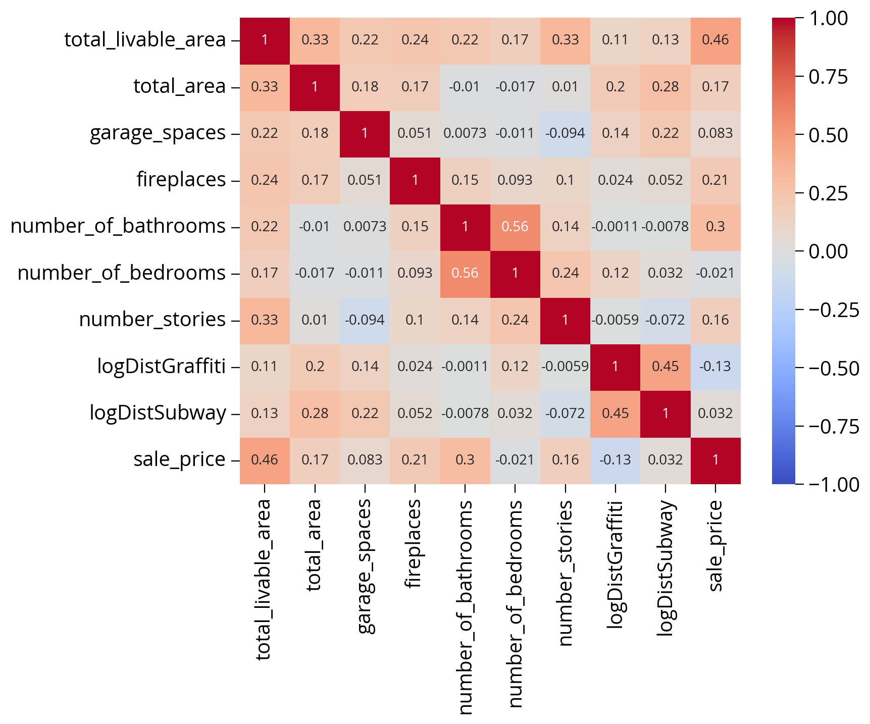

Now, let’s re-run our model…did it help?

# Numerical columns
num_cols = [
    "total_livable_area",
    "total_area",
    "garage_spaces",
    "fireplaces",
    "number_of_bathrooms",
    "number_of_bedrooms",
    "number_stories",
    "logDistGraffiti", # NEW
    "logDistSubway" # NEW
]

# Categorical columns
cat_cols = ["exterior_condition", "zip_code"]

# Set up the column transformer with two transformers
transformer = ColumnTransformer(
    transformers=[
        ("num", StandardScaler(), num_cols),
        ("cat", OneHotEncoder(handle_unknown="ignore"), cat_cols),
    ]
)

# Initialize the pipeline
# NOTE: only use 20 estimators here so it will run in a reasonable time
pipe = make_pipeline(
    transformer, RandomForestRegressor(n_estimators=20, random_state=42)
)

# Split the data 70/30
train_set, test_set = train_test_split(sales, test_size=0.3, random_state=42)

# the target labels
y_train = np.log(train_set["sale_price"])
y_test = np.log(test_set["sale_price"])

# Fit the training set
# REMINDER: use the training dataframe objects here rather than numpy array
pipe.fit(train_set, y_train);

# What's the test score?
# REMINDER: use the test dataframe rather than numpy array
pipe.score(test_set, y_test)

0.5818673189789565

A small improvement!

R-squared of ~0.53 improved to R-squared of ~0.59

How about the top 30 feature importances now?

def plot_feature_importances(pipeline, num_cols, transformer, top=20, **kwargs):
    """
    Utility function to plot the feature importances from the input
    random forest regressor.

    Parameters
    ----------
    pipeline :
        the pipeline object
    num_cols :
        list of the numerical columns
    transformer :
        the transformer preprocessing step
    top : optional
        the number of importances to plot
    **kwargs : optional
        extra keywords passed to the hvplot function
    """
    # The one-hot step
    ohe = transformer.named_transformers_["cat"]

    # One column for each category type!
    ohe_cols = ohe.get_feature_names_out()

    # Full list of columns is numerical + one-hot
    features = num_cols + list(ohe_cols)

    # The regressor
    regressor = pipeline["randomforestregressor"]

    # Create the dataframe with importances
    importance = pd.DataFrame(
        {"Feature": features, "Importance": regressor.feature_importances_}
    )

    # Sort importance in descending order and get the top
    importance = importance.sort_values("Importance", ascending=False).iloc[:top]

    # Plot
    return importance.hvplot.barh(
        x="Feature", y="Importance", flip_yaxis=True, **kwargs
    )

plot_feature_importances(pipe, num_cols, transformer, top=30, height=500)

Both new spatial features are in the top 5 in terms of importance!

Exercise: How about other spatial features?

• I’ve listed out several other types of potential sources of new distance-based features from OpenDataPhilly
• Choose a few and add new features
• Re-fit the model and evalute the performance on the test set and feature importances

Modify the get_xy_from_geometry() function to use the “centroid” of the geometry column.

Note: you can take the centroid of a Point() or Polygon() object. For a Point(), you just get the x/y coordinates back.

def get_xy_from_geometry(df):
    """
    Return a numpy array with two columns, where the 
    first holds the `x` geometry coordinate and the second 
    column holds the `y` geometry coordinate
    """
    # NEW: use the centroid.x and centroid.y to support Polygon() and Point() geometries 
    x = df.geometry.centroid.x
    y = df.geometry.centroid.y
    
    return np.column_stack((x, y)) # stack as columns

1. Universities

New feature: Distance to the nearest university/college

• Source: OpenDataPhilly
• GeoJSON URL

# Get the data
url = "https://opendata.arcgis.com/api/v3/datasets/8ad76bc179cf44bd9b1c23d6f66f57d1_0/downloads/data?format=geojson&spatialRefId=4326"
univs = gpd.read_file(url)

# Get the X/Y
univXY = get_xy_from_geometry(univs.to_crs(epsg=3857))

# Run the k nearest algorithm
nbrs = NearestNeighbors(n_neighbors=1)
nbrs.fit(univXY)
univDists, _ = nbrs.kneighbors(salesXY)

# Add the new feature
sales['logDistUniv'] = np.log10(univDists.mean(axis=1))

fig, ax = plt.subplots(figsize=(10,10), facecolor=plt.get_cmap('viridis')(0))

x = salesXY[:,0]
y = salesXY[:,1]
ax.hexbin(x, y, C=np.log10(univDists.mean(axis=1)), gridsize=60)

# Plot the city limits
city_limits.plot(ax=ax, facecolor='none', edgecolor='white', linewidth=4)

ax.set_axis_off()
ax.set_aspect("equal")
ax.set_title("Distance to Nearest University/College", fontsize=16, color='white');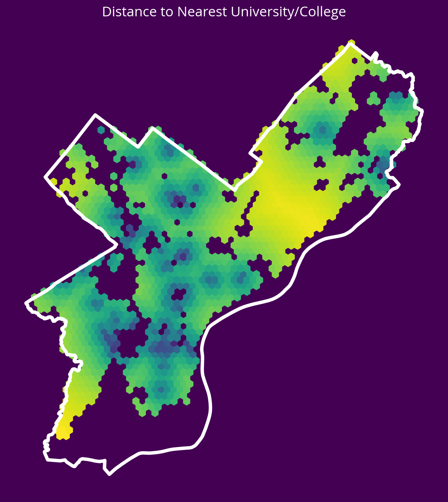

2. Parks

New feature: Distance to the nearest park centroid

• Source: OpenDataPhilly
• GeoJSON URL

Notes - The park geometries are polygons, so you’ll need to get the x and y coordinates of the park centroids and calculate the distance to these centroids. - You can use the geometry.centroid.x and geometry.centroid.y values to access these coordinates.

# Get the data
url = "https://opendata.arcgis.com/datasets/d52445160ab14380a673e5849203eb64_0.geojson"
parks = gpd.read_file(url)

# Get the X/Y
parksXY = get_xy_from_geometry(parks.to_crs(epsg=3857))

# Run the k nearest algorithm
nbrs = NearestNeighbors(n_neighbors=1)
nbrs.fit(parksXY)
parksDists, _ = nbrs.kneighbors(salesXY)

# Add the new feature
sales["logDistParks"] = np.log10(parksDists.mean(axis=1))

fig, ax = plt.subplots(figsize=(10, 10), facecolor=plt.get_cmap("viridis")(0))

x = salesXY[:, 0]
y = salesXY[:, 1]
ax.hexbin(x, y, C=np.log10(parksDists.mean(axis=1)), gridsize=60)

# Plot the city limits
city_limits.plot(ax=ax, facecolor="none", edgecolor="white", linewidth=4)

ax.set_axis_off()
ax.set_aspect("equal")
ax.set_title("Distance to Nearest Park", fontsize=16, color="white");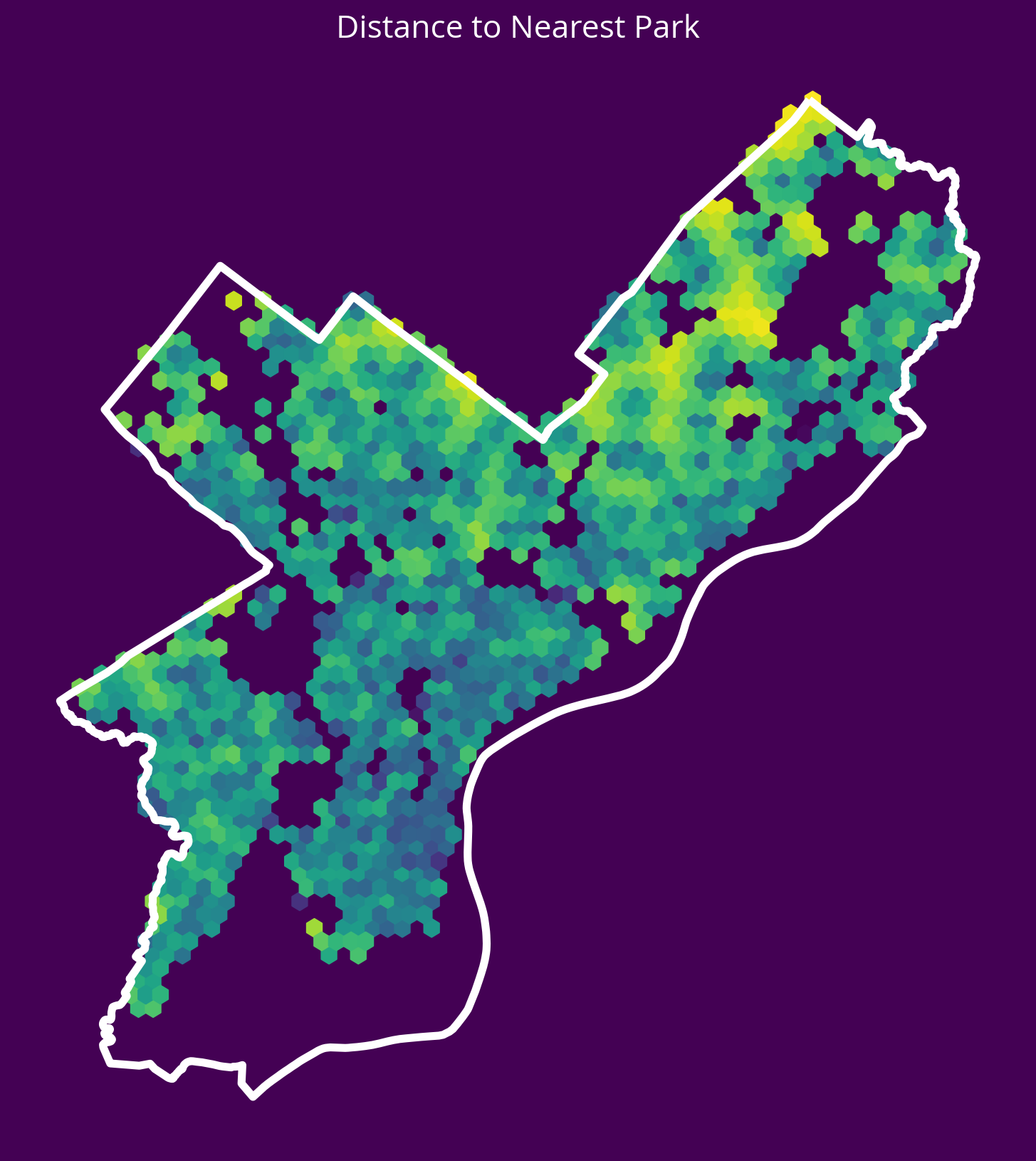

3. City Hall

New feature: Distance to City Hall.

• Source: OpenDataPhilly
• GeoJSON URL

Notes

• To identify City Hall, you’ll need to pull data where “NAME=‘City Hall’” and “FEAT_TYPE=‘Municipal Building’”
• As with the parks, the geometry will be a polygon, so you should calculate the distance to the centroid of the City Hall polygon

# Get the data
url = "http://data-phl.opendata.arcgis.com/datasets/5146960d4d014f2396cb82f31cd82dfe_0.geojson"
landmarks = gpd.read_file(url)

# Trim to City Hall
cityHall = landmarks.query("NAME == 'City Hall' and FEAT_TYPE == 'Municipal Building'")

# Get the X/Y
cityHallXY = get_xy_from_geometry(cityHall.to_crs(epsg=3857))

# Run the k nearest algorithm
nbrs = NearestNeighbors(n_neighbors=1)
nbrs.fit(cityHallXY)
cityHallDist, _ = nbrs.kneighbors(salesXY)

# Add the new feature
sales["logDistCityHall"] = np.log10(cityHallDist.mean(axis=1))

fig, ax = plt.subplots(figsize=(10, 10), facecolor=plt.get_cmap("viridis")(0))

x = salesXY[:, 0]
y = salesXY[:, 1]
ax.hexbin(x, y, C=np.log10(cityHallDist.mean(axis=1)), gridsize=60)

# Plot the city limits
city_limits.plot(ax=ax, facecolor="none", edgecolor="white", linewidth=4)

ax.set_axis_off()
ax.set_aspect("equal")
ax.set_title("Distance to City Hall", fontsize=16, color="white");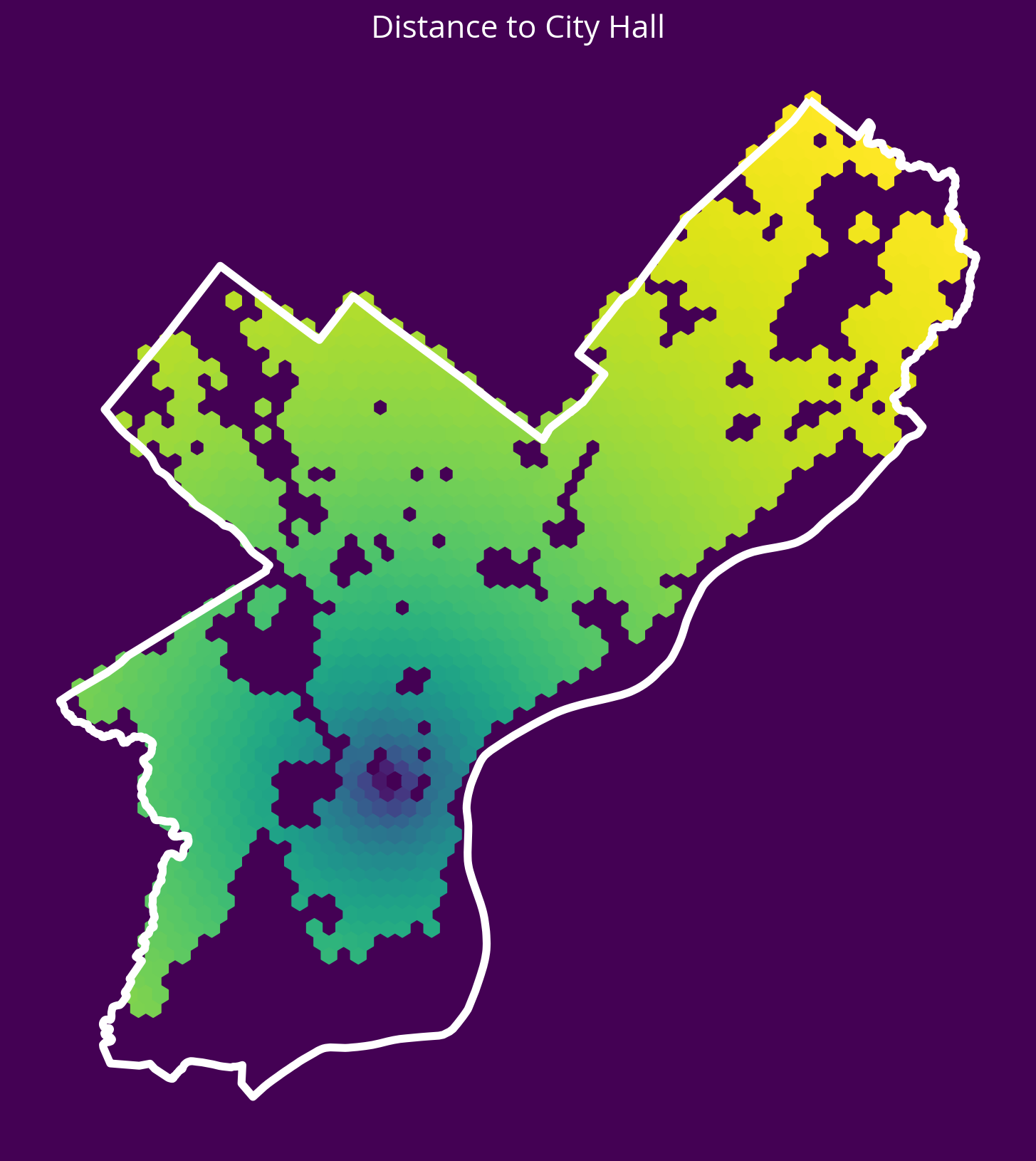

4. Residential Construction Permits

New feature: Distance to the 5 nearest residential construction permits from 2022

• Source: OpenDataPhilly
• CARTO table name: “permits”

Notes

• You can pull new construction permits only by selecting where permitdescription equals ‘RESIDENTRIAL CONSTRUCTION PERMIT’
• You can select permits from only 2022 using the permitissuedate column

# Table name
table_name = "permits"

# Where clause
where = "permitissuedate >= '2022-01-01' AND permitissuedate < '2023-01-01'"
where = where + " AND permitdescription='RESIDENTIAL BUILDING PERMIT'"

# Query
permits = get_carto_data(table_name, where=where)

# Remove missing
not_missing = ~permits.geometry.is_empty & permits.geometry.notna()
permits = permits.loc[not_missing]

# Get the X/Y
permitsXY = get_xy_from_geometry(permits.to_crs(epsg=3857))

# Run the k nearest algorithm
nbrs = NearestNeighbors(n_neighbors=5)
nbrs.fit(permitsXY)
permitsDist, _ = nbrs.kneighbors(salesXY)

# Add the new feature
sales["logDistPermits"] = np.log10(permitsDist.mean(axis=1))

/var/folders/49/ntrr94q12xd4rq8hqdnx96gm0000gn/T/ipykernel_96911/3972340687.py:12: UserWarning: GeoSeries.notna() previously returned False for both missing (None) and empty geometries. Now, it only returns False for missing values. Since the calling GeoSeries contains empty geometries, the result has changed compared to previous versions of GeoPandas.
Given a GeoSeries 's', you can use '~s.is_empty & s.notna()' to get back the old behaviour.

To further ignore this warning, you can do: 
import warnings; warnings.filterwarnings('ignore', 'GeoSeries.notna', UserWarning)
  not_missing = ~permits.geometry.is_empty & permits.geometry.notna()

fig, ax = plt.subplots(figsize=(10, 10), facecolor=plt.get_cmap("viridis")(0))

x = salesXY[:, 0]
y = salesXY[:, 1]
ax.hexbin(x, y, C=np.log10(permitsDist.mean(axis=1)), gridsize=60)

# Plot the city limits
city_limits.plot(ax=ax, facecolor="none", edgecolor="white", linewidth=4)

ax.set_axis_off()
ax.set_aspect("equal")
ax.set_title("Distance to 5 Closest Building Permits", fontsize=16, color="white");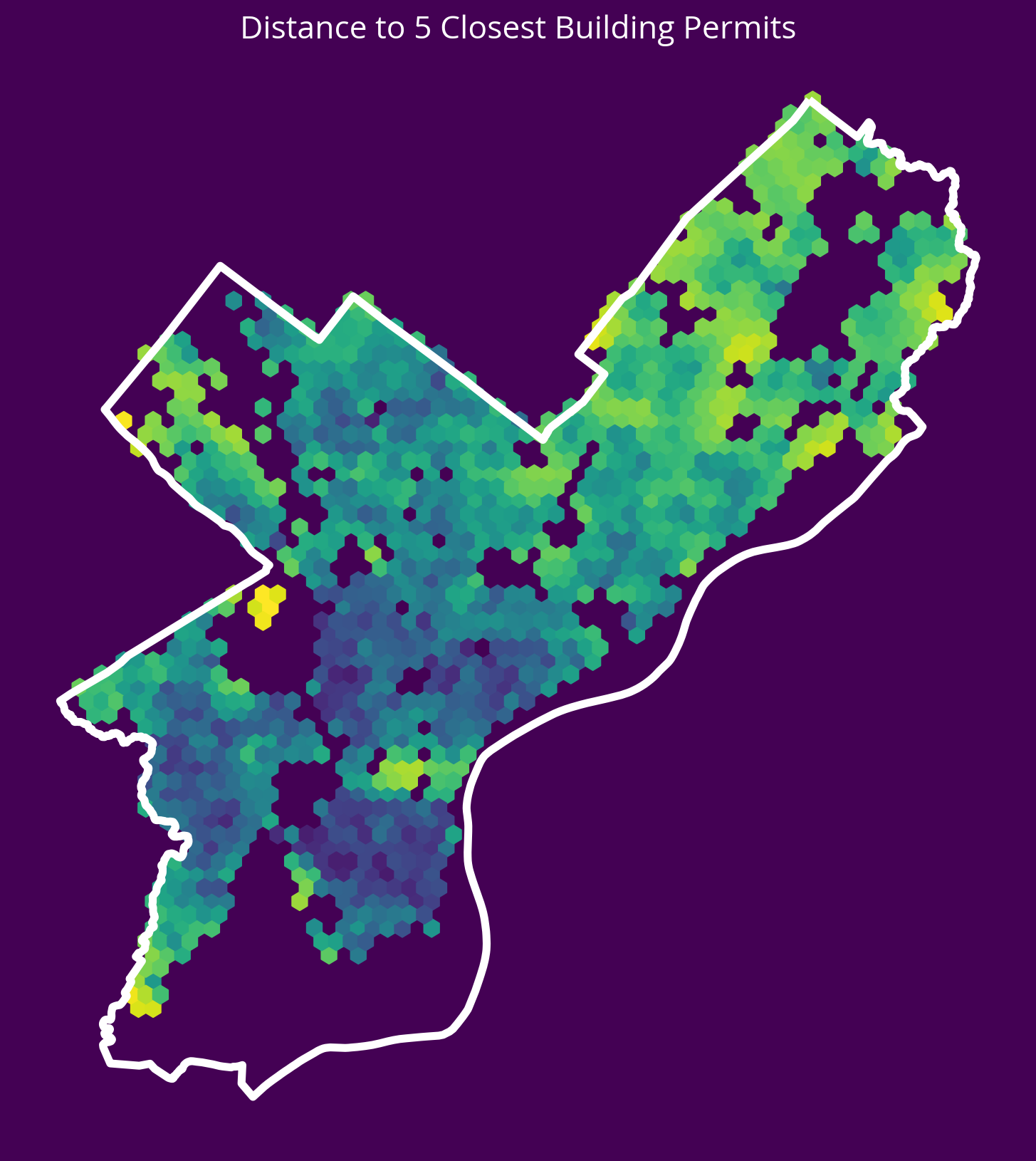

5. Aggravated Assaults

New feature: Distance to the 5 nearest aggravated assaults in 2022

• Source: OpenDataPhilly
• CARTO table name: “incidents_part1_part2”

Notes

• You can pull aggravated assaults only by selecting where Text_General_Code equals ‘Aggravated Assault No Firearm’ or ‘Aggravated Assault Firearm’
• You can select crimes from only 2022 using the dispatch_date column

# Table name
table_name = "incidents_part1_part2"

# Where selection
where = "dispatch_date >= '2022-01-01' AND dispatch_date < '2023-01-01'"
where = where + " AND Text_General_Code IN ('Aggravated Assault No Firearm', 'Aggravated Assault Firearm')"

# Query
assaults = get_carto_data(table_name, where=where)

# Remove missing 
not_missing = ~assaults.geometry.is_empty & assaults.geometry.notna()
assaults = assaults.loc[not_missing]
    
# Get the X/Y
assaultsXY = get_xy_from_geometry(assaults.to_crs(epsg=3857))

# Run the k nearest algorithm
nbrs = NearestNeighbors(n_neighbors=5)
nbrs.fit(assaultsXY)
assaultDists, _ = nbrs.kneighbors(salesXY)

# Add the new feature
sales['logDistAssaults'] = np.log10(assaultDists.mean(axis=1))

fig, ax = plt.subplots(figsize=(10, 10), facecolor=plt.get_cmap("viridis")(0))

x = salesXY[:, 0]
y = salesXY[:, 1]
ax.hexbin(x, y, C=np.log10(assaultDists.mean(axis=1)), gridsize=60)

# Plot the city limits
city_limits.plot(ax=ax, facecolor="none", edgecolor="white", linewidth=4)

ax.set_axis_off()
ax.set_aspect("equal")
ax.set_title("Distance to 5 Closest Assaults", fontsize=16, color="white");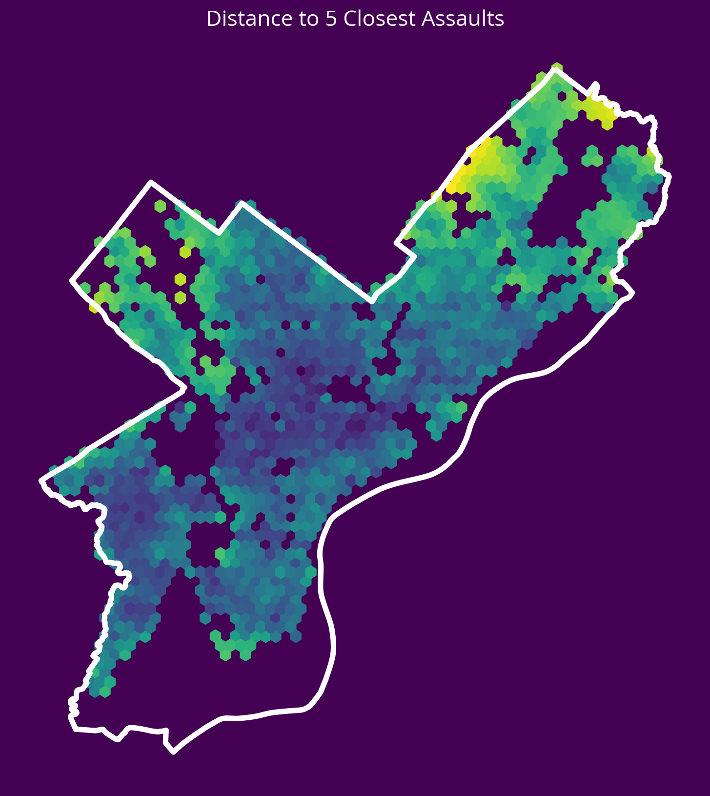

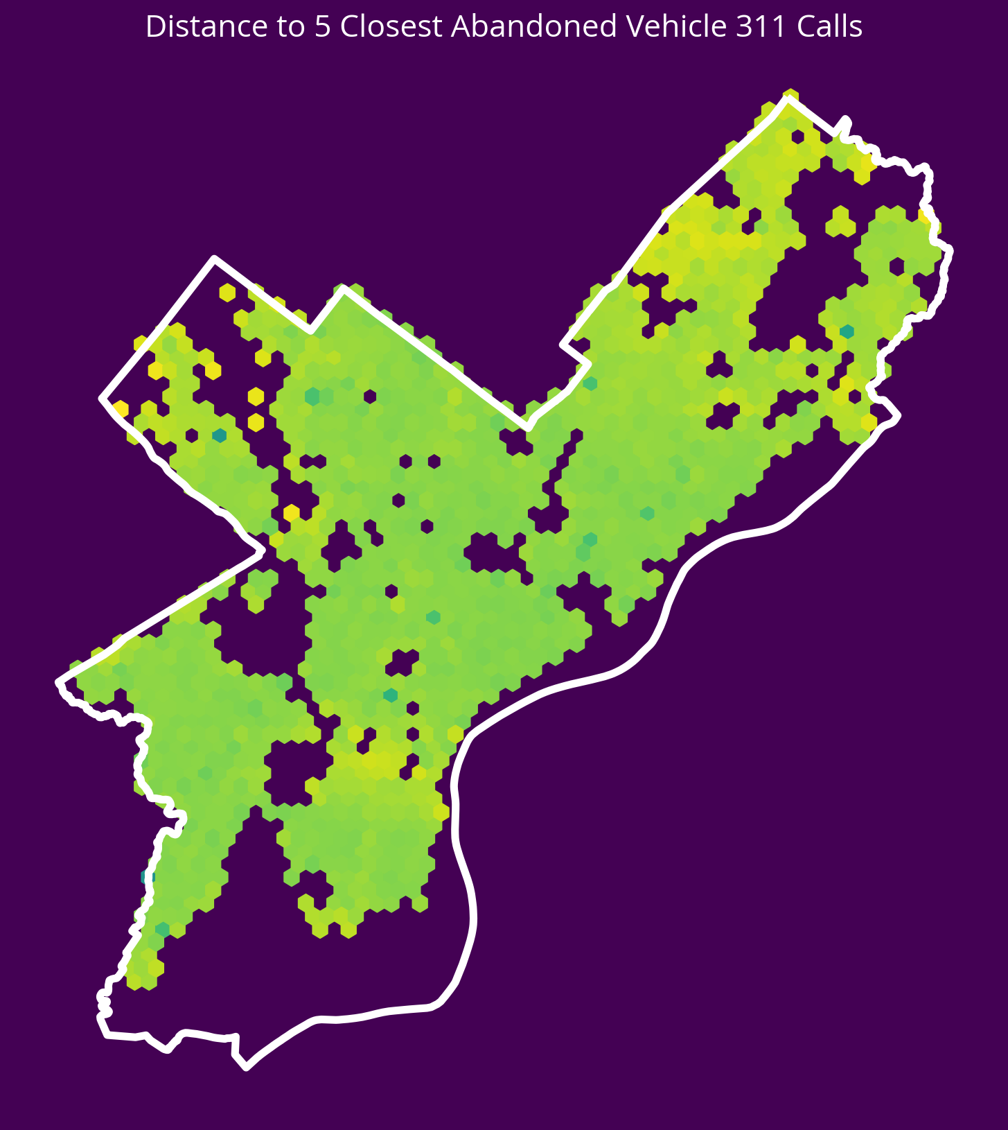
6. Abandonded Vehicle 311 Calls

New feature: Distance to the 5 nearest abandoned vehicle 311 calls in 2022

• Source: OpenDataPhilly
• CARTO table name: “public_cases_fc”

Notes

• You can pull abandonded vehicle calls only by selecting where service_name equals ‘Abandoned Vehicle’
• You can select crimes from only 2022 using the requested_datetime column

# Table name
table_name = "public_cases_fc"

# Where selection
where = "requested_datetime >= '2022-01-01' AND requested_datetime < '2023-01-01'"
where = "service_name = 'Abandoned Vehicle'"

# Query
cars = get_carto_data(table_name, where=where)

# Remove missing
not_missing = ~cars.geometry.is_empty & cars.geometry.notna()
cars = cars.loc[not_missing]

# Get the X/Y
carsXY = get_xy_from_geometry(cars.to_crs(epsg=3857))

# Run the k nearest algorithm
nbrs = NearestNeighbors(n_neighbors=5)
nbrs.fit(carsXY)
carDists, _ = nbrs.kneighbors(salesXY)

# Handle any sales that have 0 distances
carDists[carDists == 0] = 1e-5  # a small, arbitrary value

# Add the new feature
sales["logDistCars"] = np.log10(carDists.mean(axis=1))

fig, ax = plt.subplots(figsize=(10, 10), facecolor=plt.get_cmap("viridis")(0))

x = salesXY[:, 0]
y = salesXY[:, 1]
ax.hexbin(x, y, C=np.log10(carDists.mean(axis=1)), gridsize=60)

# Plot the city limits
city_limits.plot(ax=ax, facecolor="none", edgecolor="white", linewidth=4)

ax.set_axis_off()
ax.set_aspect("equal")
ax.set_title(
    "Distance to 5 Closest Abandoned Vehicle 311 Calls", fontsize=16, color="white"
);